

12
Inf
9.3
1.2
1.0
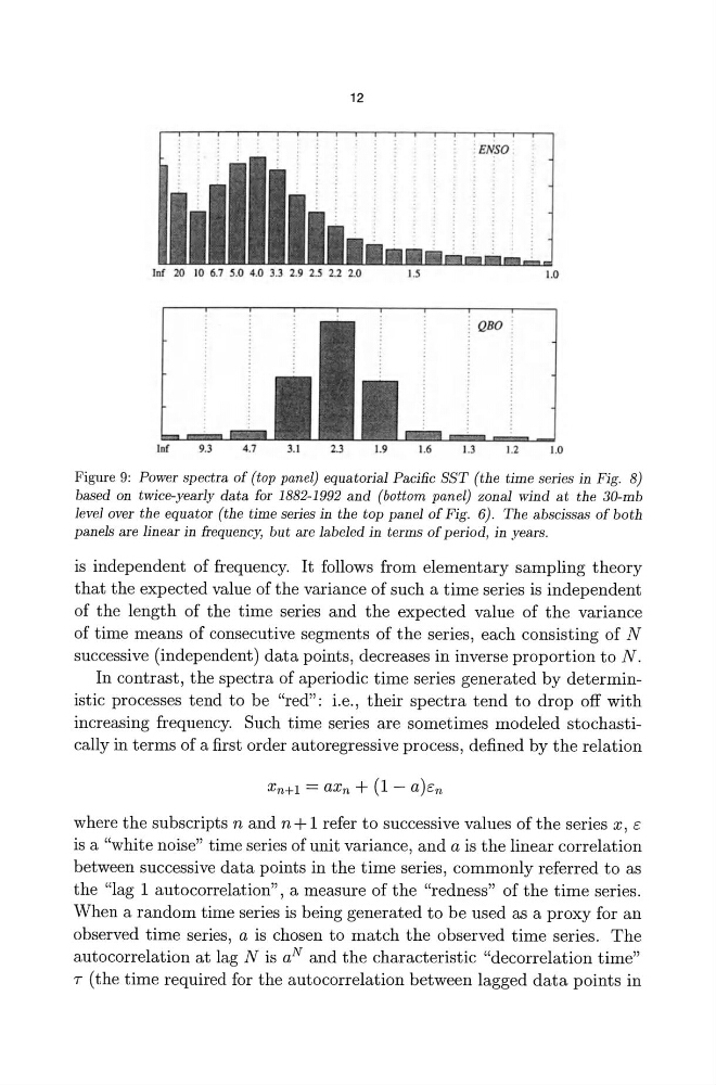
Figure 9: Power spectra of (top panel) equatorial Pacific SST (the time series in Fig. 8)
based on twice-yearly data for 1882-1992 and (bottom panel) zonal wind at the 30-mb
level over the equator (the time series in the top panel of Fig. 6). The abscissas of both
panels are linear in frequency, but are labeled in terms of period, in years.
is independent of frequency. It follows from elementary sampling theory
that the expected value of the variance of such a time series is independent
of the length of the time series and the expected value of the variance
of time means of consecutive segments of the series, each consisting of N
successive (independent) data points, decreases in inverse proportion to N.
In contrast, the spectra of aperiodic time series generated by deterministic processes tend to be "red": i.e., their spectra tend to drop off with
increasing frequency. Such time series are sometimes modeled stochastically in terms of a first order autoregressive process, defined by the relation
Xn+l = aXn + (1 - a)C:n
where the subscripts nand n + 1 refer to successive values of the series x, c:
is a "white noise" time series of unit variance, and a is the linear correlation
between successive data points in the time series, commonly referred to as
the "lag 1 autocorrelation", a measure of the "redness" of the time series.
When a random time series is being generated to be used as a proxy for an
observed time series, a is chosen to match the observed time series. The
autocorrelation at lag N is a N and the characteristic "decorrelation time"
T (the time required for the autocorrelation between lagged data points in
Inf
9.3
1.2
1.0
Figure 9: Power spectra of (top panel) equatorial Pacific SST (the time series in Fig. 8)
based on twice-yearly data for 1882-1992 and (bottom panel) zonal wind at the 30-mb
level over the equator (the time series in the top panel of Fig. 6). The abscissas of both
panels are linear in frequency, but are labeled in terms of period, in years.
is independent of frequency. It follows from elementary sampling theory
that the expected value of the variance of such a time series is independent
of the length of the time series and the expected value of the variance
of time means of consecutive segments of the series, each consisting of N
successive (independent) data points, decreases in inverse proportion to N.
In contrast, the spectra of aperiodic time series generated by deterministic processes tend to be "red": i.e., their spectra tend to drop off with
increasing frequency. Such time series are sometimes modeled stochastically in terms of a first order autoregressive process, defined by the relation
Xn+l = aXn + (1 - a)C:n
where the subscripts nand n + 1 refer to successive values of the series x, c:
is a "white noise" time series of unit variance, and a is the linear correlation
between successive data points in the time series, commonly referred to as
the "lag 1 autocorrelation", a measure of the "redness" of the time series.
When a random time series is being generated to be used as a proxy for an
observed time series, a is chosen to match the observed time series. The
autocorrelation at lag N is a N and the characteristic "decorrelation time"
T (the time required for the autocorrelation between lagged data points in