

110
>" 10 -.-a)-------------.
c:
w
Z
W
5
..J
«
Io
IO+-~~~-:;-:-:-~~~~~
o 5 1 0 15 20 25 30 35 40
N WAVE NUMBER
>" 10 " l . ' " : b ) - - - - - - - - - - - ,
c:
W
Z
W 5
..J
«
Io
IO-t-l..;:;:;...:r;,-,..,.,.,.,,.,...,..,.,..,..,.,..,..,....,..,."'TT"'"""""',.,..,..,..,..l
o 5 1 0 15 20 25 30 35 40
N WAVE NUMBER
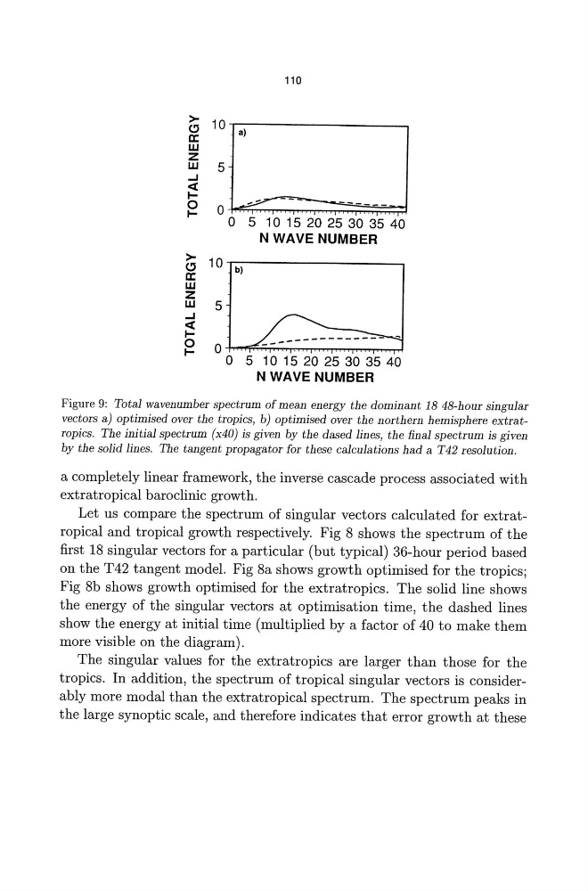
Figure 9: Total wavenumber spectrum of mean energy the dominant 18 48-hour singular
vectors a) optimised over the tropics, b) optimised over the northern hemisphere extratTOpics. The initial spectrum (x40) is given by the dased lines, the final spectrum is given
by the solid lines. The tangent propagator for these calculations had a T42 resolution.
a completely linear framework, the inverse cascade process associated with
extratropical baroclinic growth.
Let us compare the spectrum of singular vectors calculated for extratropical and tropical growth respectively. Fig 8 shows the spectrum of the
first 18 singular vectors for a particular (but typical) 36-hour period based
on the T42 tangent model. Fig 8a shows growth optimised for the tropics;
Fig 8b shows growth optimised for the extratropics. The solid line shows
the energy of the singular vectors at optimisation time, the dashed lines
show the energy at initial time (multiplied by a factor of 40 to make them
more visible on the diagram).
The singular values for the extratropics are larger than those for the
tropics. In addition, the spectrum of tropical singular vectors is considerably more modal than the extratropical spectrum. The spectrum peaks in
the large synoptic scale, and therefore indicates that error growth at these
>" 10 -.-a)-------------.
c:
w
Z
W
5
..J
«
Io
IO+-~~~-:;-:-:-~~~~~
o 5 1 0 15 20 25 30 35 40
N WAVE NUMBER
>" 10 " l . ' " : b ) - - - - - - - - - - - ,
c:
W
Z
W 5
..J
«
Io
IO-t-l..;:;:;...:r;,-,..,.,.,.,,.,...,..,.,..,..,.,..,..,....,..,."'TT"'"""""',.,..,..,..,..l
o 5 1 0 15 20 25 30 35 40
N WAVE NUMBER
Figure 9: Total wavenumber spectrum of mean energy the dominant 18 48-hour singular
vectors a) optimised over the tropics, b) optimised over the northern hemisphere extratTOpics. The initial spectrum (x40) is given by the dased lines, the final spectrum is given
by the solid lines. The tangent propagator for these calculations had a T42 resolution.
a completely linear framework, the inverse cascade process associated with
extratropical baroclinic growth.
Let us compare the spectrum of singular vectors calculated for extratropical and tropical growth respectively. Fig 8 shows the spectrum of the
first 18 singular vectors for a particular (but typical) 36-hour period based
on the T42 tangent model. Fig 8a shows growth optimised for the tropics;
Fig 8b shows growth optimised for the extratropics. The solid line shows
the energy of the singular vectors at optimisation time, the dashed lines
show the energy at initial time (multiplied by a factor of 40 to make them
more visible on the diagram).
The singular values for the extratropics are larger than those for the
tropics. In addition, the spectrum of tropical singular vectors is considerably more modal than the extratropical spectrum. The spectrum peaks in
the large synoptic scale, and therefore indicates that error growth at these