

CHAPTER 1 • The Carbonate System in Marine Environments
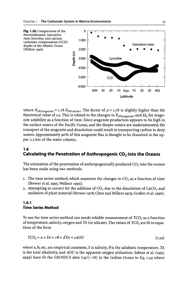
Fig. 1.20. Comparisons of the
thermodynamic saturation
state, lysocline, and calcium
carbonate compensation (CCD)
depths in the Atlantic Ocean
(Millero 1996)
g
.r:
C.
0
• • •
1000
2000
3000
4000
5000
33
• •
•
Saturation state
• • • • •
6000 '------'-_...L------"_--'--_L-...--l._--'---_-'----------'----'
40N 30 20 10 Equ. 10 20 30 40S
Lattitude
where KSP(aragonite) = 1.78 KSP(calcite)' The factor of p = 1.78 is slightly higher than the
theoretical value of 1.5. This is related to the changes in KSP(aragonite) and Q A for aragonite solubility as a function of time. Since aragonite production appears to be high in
the surface waters of the Pacific Ocean, and the deeper waters are undersaturated, the
transport of the aragonite and dissolution could result in transporting carbon to deep
waters. Approximately 90% of this aragonite flux is thought to be dissolved in the upper 2.2 km of the water column.
1.6
Calculating the Penetration of Anthropogenic CO 2 into the Oceans
The estimation of the penetration of anthropogenically produced CO2 into the oceans
has been made using two methods:
1. The time series method, which examines the changes in CO2 as a function of time
(Brewer et al. 1995; Wallace 1995);
2. Attempting to correct for the addition of CO2 due to the dissolution of CaC03 and
oxidation of plant material (Brewer 1978; Chen and Millero 1979; Gruber et al. 1996).
1.6.1
Time Series Method
To use the time series method one needs reliable measurement of Te0 2 as a function
of temperature, salinity, oxygen and TA (or silicate). The values of Te0 2 are fit to equations of the form
Te02 = a + bS + c(}+ dTA + eAOU
where a, b, etc. are empirical constants, S is salinity, () is the adiabatic temperature, TA
is the total alkalinity, and AOU is the apparent oxygen utilization. Sabine et al. (1997,
1999) have fit the GEOSECS data (1977-78) in the Indian Ocean to Eq. 1.34 where
Fig. 1.20. Comparisons of the
thermodynamic saturation
state, lysocline, and calcium
carbonate compensation (CCD)
depths in the Atlantic Ocean
(Millero 1996)
g
.r:
C.
0
• • •
1000
2000
3000
4000
5000
33
• •
•
Saturation state
• • • • •
6000 '------'-_...L------"_--'--_L-...--l._--'---_-'----------'----'
40N 30 20 10 Equ. 10 20 30 40S
Lattitude
where KSP(aragonite) = 1.78 KSP(calcite)' The factor of p = 1.78 is slightly higher than the
theoretical value of 1.5. This is related to the changes in KSP(aragonite) and Q A for aragonite solubility as a function of time. Since aragonite production appears to be high in
the surface waters of the Pacific Ocean, and the deeper waters are undersaturated, the
transport of the aragonite and dissolution could result in transporting carbon to deep
waters. Approximately 90% of this aragonite flux is thought to be dissolved in the upper 2.2 km of the water column.
1.6
Calculating the Penetration of Anthropogenic CO 2 into the Oceans
The estimation of the penetration of anthropogenically produced CO2 into the oceans
has been made using two methods:
1. The time series method, which examines the changes in CO2 as a function of time
(Brewer et al. 1995; Wallace 1995);
2. Attempting to correct for the addition of CO2 due to the dissolution of CaC03 and
oxidation of plant material (Brewer 1978; Chen and Millero 1979; Gruber et al. 1996).
1.6.1
Time Series Method
To use the time series method one needs reliable measurement of Te0 2 as a function
of temperature, salinity, oxygen and TA (or silicate). The values of Te0 2 are fit to equations of the form
Te02 = a + bS + c(}+ dTA + eAOU
where a, b, etc. are empirical constants, S is salinity, () is the adiabatic temperature, TA
is the total alkalinity, and AOU is the apparent oxygen utilization. Sabine et al. (1997,
1999) have fit the GEOSECS data (1977-78) in the Indian Ocean to Eq. 1.34 where