

76
4. Finite Volume Methods
4.4 Interpolation and Differentiation Practices
The approximations to the integrals require the values of variables a t locations other than computational nodes (CV centers). The integrand, denoted
in the previous sections by f , involves the product of several variables and/or
variable gradients at those locations: fC = pdv. n for the convective flux and
f d = Fgrad q?~ . n for the diffusive flux. We assume that the velocity field
and the fluid properties p and r are known at all locations. To calculate
the convective and diffusive fluxes, the value of and its gradient normal to
the cell face a t one or more locations on the CV surface are needed. Volume
integrals of the source terms may also require these values. They have t o be
expressed in terms of the nodal values by interpolation. Numerous possibilities are available; we shall mention a few that are most commonly used. In
particular we shall show how the value of and its normal derivative a t cell
face 'e' can be approximated.
4.4.1 Upwind Interpolation (UDS)
Approximating 4, by its value a t the node upstream of 'e' is equivalent to
using a backward- or forward-difference approximation for the first derivative (depending on the flow direction), hence the name upwind differencing
scheme (UDS) for this approximation. In UDS, 4, is approximated as:
P if (v . n), > 0 ;
me={' 4~ if . (v . n), < 0 .
This is the only approximation that unconditionally satisfies the boundedness
criterion i.e. it will never yield oscillatory solutions. However, it achieves this
by being numerically diffusive. This was shown in the preceding chapter and
will be shown again below.
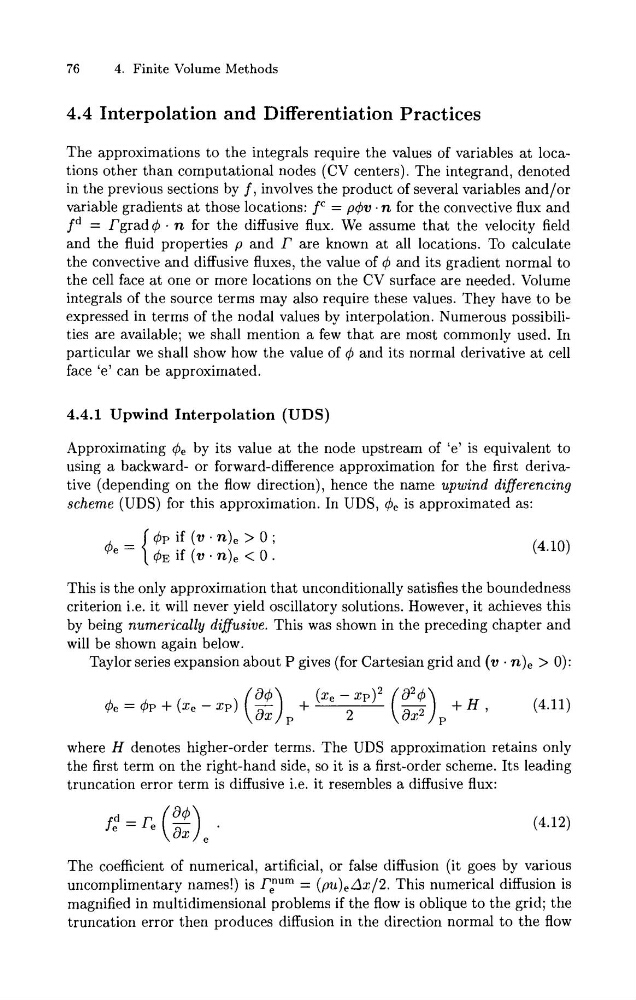
Taylor series expansion about P gives (for Cartesian grid and (v . n), > 0):
where H denotes higher-order terms. The UDS approximation retains only
the first term on the right-hand side, so it is a first-order scheme. Its leading
truncation error term is diffusive i.e. it resembles a diffusive flux:
The coefficient of numerical, artificial, or false diffusion (it goes by various
uncomplimentary names!) is r,"um = (pu),Ax/2. This numerical diffusion is
magnified in multidimensional problems if the flow is oblique to the grid; the
truncation error then produces diffusion in the direction normal to the flow
4. Finite Volume Methods
4.4 Interpolation and Differentiation Practices
The approximations to the integrals require the values of variables a t locations other than computational nodes (CV centers). The integrand, denoted
in the previous sections by f , involves the product of several variables and/or
variable gradients at those locations: fC = pdv. n for the convective flux and
f d = Fgrad q?~ . n for the diffusive flux. We assume that the velocity field
and the fluid properties p and r are known at all locations. To calculate
the convective and diffusive fluxes, the value of and its gradient normal to
the cell face a t one or more locations on the CV surface are needed. Volume
integrals of the source terms may also require these values. They have t o be
expressed in terms of the nodal values by interpolation. Numerous possibilities are available; we shall mention a few that are most commonly used. In
particular we shall show how the value of and its normal derivative a t cell
face 'e' can be approximated.
4.4.1 Upwind Interpolation (UDS)
Approximating 4, by its value a t the node upstream of 'e' is equivalent to
using a backward- or forward-difference approximation for the first derivative (depending on the flow direction), hence the name upwind differencing
scheme (UDS) for this approximation. In UDS, 4, is approximated as:
P if (v . n), > 0 ;
me={' 4~ if . (v . n), < 0 .
This is the only approximation that unconditionally satisfies the boundedness
criterion i.e. it will never yield oscillatory solutions. However, it achieves this
by being numerically diffusive. This was shown in the preceding chapter and
will be shown again below.
Taylor series expansion about P gives (for Cartesian grid and (v . n), > 0):
where H denotes higher-order terms. The UDS approximation retains only
the first term on the right-hand side, so it is a first-order scheme. Its leading
truncation error term is diffusive i.e. it resembles a diffusive flux:
The coefficient of numerical, artificial, or false diffusion (it goes by various
uncomplimentary names!) is r,"um = (pu),Ax/2. This numerical diffusion is
magnified in multidimensional problems if the flow is oblique to the grid; the
truncation error then produces diffusion in the direction normal to the flow