

4.3 Approximation of Volume Integrals
75
4.3 Approximat ion of Volume Integrals
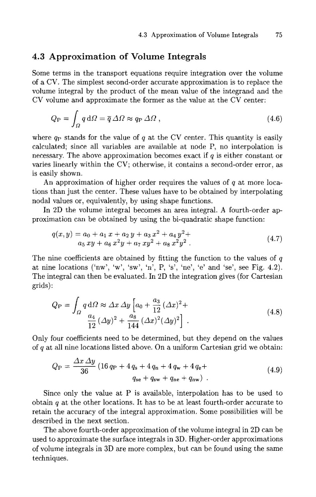
Some terms in the transport equations require integration over the volume
of a CV. The simplest second-order accurate approximation is to replace the
volume integral by the product of the mean value of the integrand and the
CV volume and approximate the former as the value at the CV center:
where qp stands for the value of q a t the CV center. This quantity is easily
calculated; since all variables are available at node P, no interpolation is
necessary. The above approximation becomes exact if q is either constant or
varies linearly within the CV; otherwise, it contains a second-order error, as
is easily shown.
An approximation of higher order requires the values of q a t more locations than just the center. These values have to be obtained by interpolating
nodal values or, equivalently, by using shape functions.
In 2D the volume integral becomes an area integral. A fourth-order approximation can be obtained by using the bi-quadratic shape function:
The nine coefficients are obtained by fitting the function to the values of q
a t nine locations ('nw', 'w', 'sw', 'n', P, 's', 'ne', 'e' and 'se', see Fig. 4.2).
The integral can then be evaluated. In 2D the integration gives (for Cartesian
grids) :
Only four coefficients need to be determined, but they depend on the values
of q a t all nine locations listed above. On a uniform Cartesian grid we obtain:
Since only the value a t P is available, interpolation has to be used to
obtain q a t the other locations. It has to be at least fourth-order accurate to
retain the accuracy of the integral approximation. Some possibilities will be
described in the next section.
The above fourth-order approximation of the volume integral in 2D can be
used to approximate the surface integrals in 3D. Higher-order approximations
of volume integrals in 3D are more complex, but can be found using the same
techniques.
75
4.3 Approximat ion of Volume Integrals
Some terms in the transport equations require integration over the volume
of a CV. The simplest second-order accurate approximation is to replace the
volume integral by the product of the mean value of the integrand and the
CV volume and approximate the former as the value at the CV center:
where qp stands for the value of q a t the CV center. This quantity is easily
calculated; since all variables are available at node P, no interpolation is
necessary. The above approximation becomes exact if q is either constant or
varies linearly within the CV; otherwise, it contains a second-order error, as
is easily shown.
An approximation of higher order requires the values of q a t more locations than just the center. These values have to be obtained by interpolating
nodal values or, equivalently, by using shape functions.
In 2D the volume integral becomes an area integral. A fourth-order approximation can be obtained by using the bi-quadratic shape function:
The nine coefficients are obtained by fitting the function to the values of q
a t nine locations ('nw', 'w', 'sw', 'n', P, 's', 'ne', 'e' and 'se', see Fig. 4.2).
The integral can then be evaluated. In 2D the integration gives (for Cartesian
grids) :
Only four coefficients need to be determined, but they depend on the values
of q a t all nine locations listed above. On a uniform Cartesian grid we obtain:
Since only the value a t P is available, interpolation has to be used to
obtain q a t the other locations. It has to be at least fourth-order accurate to
retain the accuracy of the integral approximation. Some possibilities will be
described in the next section.
The above fourth-order approximation of the volume integral in 2D can be
used to approximate the surface integrals in 3D. Higher-order approximations
of volume integrals in 3D are more complex, but can be found using the same
techniques.