

12.4 Moving Grids
373
12.3 Flows With Variable Fluid Properties
Although we have dealt mainly with incompressible flows, the density, viscosity, and other fluid properties have been kept inside the differential operators.
This allows the discretization and solution methods presented in the preceding chapters to be used to solve problems with variable fluid properties.
The variation in fluid properties is usually caused by temperature variation; pressure variation also affects the change of density. This kind of variation was considered in Chap. 10, where we dealt with compressible flows.
However, there are many cases in which the pressure does not change substantially, but the temperature and/or concentration of solutes can cause large
variation in fluid properties. Examples are gas flows a t reduced pressure, flows
in liquid metals (crystal growth, solidification and melting problems, etc.),
and environmental flows of fluids stratified by dissolved salt.
Variations in density, viscosity, Prandtl number, and specific heat increase
the non-linearity of the equations. The sequential solution method can be
applied to these flows in the much the same way they are applied to flows with
variable temperature. One recalculates the fluid properties after each outer
iteration and treats them as known during the next outer iteration. If the
property variation is significant the convergence may be slowed considerably.
For steady flows, the multigrid method can result in a substantial speed-up;
see Durst et al. (1992) for an example of application to metalorganic chemical
vapor deposition problems, and Kadinski and PeriC (1995) for application to
problems involving thermal radiation.
Flows in the atmosphere and the oceans are special examples of variable
density flows; they are discussed later.
12.4 Moving Grids
In many application areas the solution domain changes with time due to the
movement of boundaries. The movement is determined either by external
effects (as in piston-driven flows) or by calculation as part of the solution
(for example, in free-surface flows). In either case, the grid has to move to
accommodate the changing boundary. If the coordinate system remains fixed
and the Cartesian velocity components are used, the only change in the conservation equations is the appearance of the relative velocity in convective
terms; see Sect. 1.2. We describe here briefly how the equations for a moving
grid system can be derived.
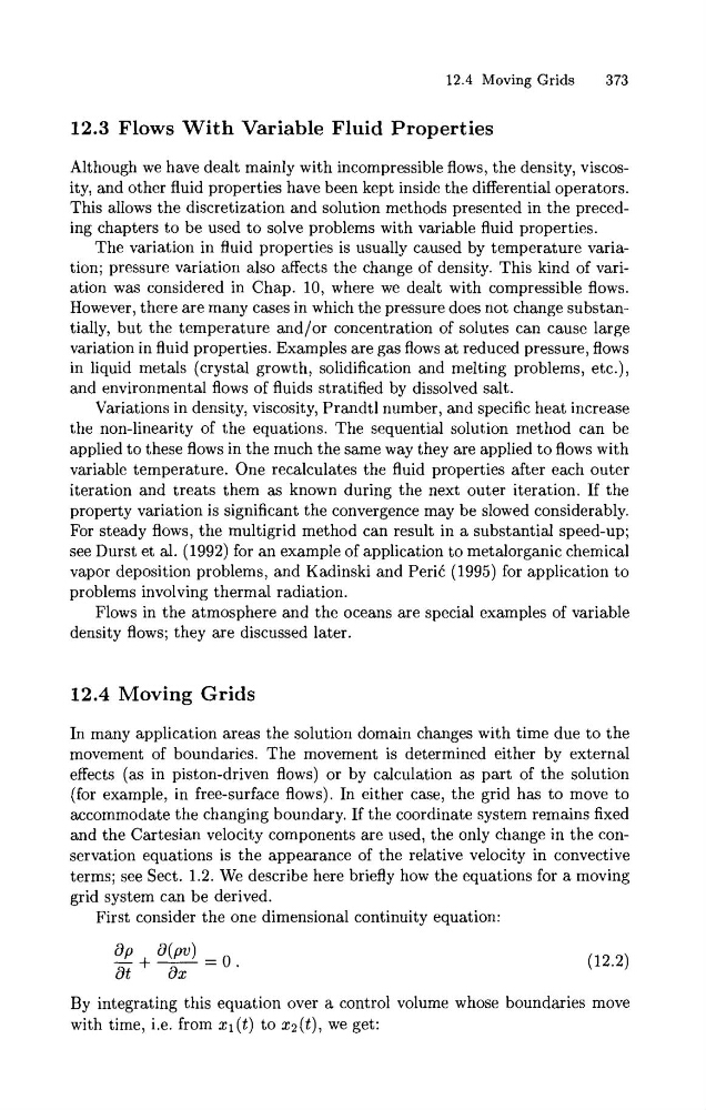
First consider the one dimensional continuity equation:
By integrating this equation over a control volume whose boundaries move
with time, i.e. from x1 (t) to x2(t), we get:
373
12.3 Flows With Variable Fluid Properties
Although we have dealt mainly with incompressible flows, the density, viscosity, and other fluid properties have been kept inside the differential operators.
This allows the discretization and solution methods presented in the preceding chapters to be used to solve problems with variable fluid properties.
The variation in fluid properties is usually caused by temperature variation; pressure variation also affects the change of density. This kind of variation was considered in Chap. 10, where we dealt with compressible flows.
However, there are many cases in which the pressure does not change substantially, but the temperature and/or concentration of solutes can cause large
variation in fluid properties. Examples are gas flows a t reduced pressure, flows
in liquid metals (crystal growth, solidification and melting problems, etc.),
and environmental flows of fluids stratified by dissolved salt.
Variations in density, viscosity, Prandtl number, and specific heat increase
the non-linearity of the equations. The sequential solution method can be
applied to these flows in the much the same way they are applied to flows with
variable temperature. One recalculates the fluid properties after each outer
iteration and treats them as known during the next outer iteration. If the
property variation is significant the convergence may be slowed considerably.
For steady flows, the multigrid method can result in a substantial speed-up;
see Durst et al. (1992) for an example of application to metalorganic chemical
vapor deposition problems, and Kadinski and PeriC (1995) for application to
problems involving thermal radiation.
Flows in the atmosphere and the oceans are special examples of variable
density flows; they are discussed later.
12.4 Moving Grids
In many application areas the solution domain changes with time due to the
movement of boundaries. The movement is determined either by external
effects (as in piston-driven flows) or by calculation as part of the solution
(for example, in free-surface flows). In either case, the grid has to move to
accommodate the changing boundary. If the coordinate system remains fixed
and the Cartesian velocity components are used, the only change in the conservation equations is the appearance of the relative velocity in convective
terms; see Sect. 1.2. We describe here briefly how the equations for a moving
grid system can be derived.
First consider the one dimensional continuity equation:
By integrating this equation over a control volume whose boundaries move
with time, i.e. from x1 (t) to x2(t), we get: