

346
11. Efficiency and Accuracy Improvement
above equation are the corresponding terms on the right hand side. If the
fine-grid residual is zero, the solution will be oh = &h.
Only if the residual on the fine grid is non-zero, will the coarse-grid approximation change from its initial value (since the problem is non-linear, the
coefficient matrix and the source term also change, which is why these terms
carry a A symbol). Once the solution on the coarse grid is obtained (within a
certain tolerance), the correction
is transferred by interpolation ('prolonged') to the fine grid and added to the
existing solution 4 r . With this correction, much of the low-frequency error in
the solution on the fine grid is removed, saving a lot of iterations on the fine
grid. This process is continued until the solution on fine grid is converged.
Richardson extrapolation may then be used to obtain an improved starting
guess for the next finer grid, and a three level V-cycle is initiated, and so on.
For structured grids, simple bilinear (in 2D) or trilinear (in 3D) interpolation is usually used t o transfer variable values from fine to coarse grids and
corrections from coarse to fine grids. Although more complex interpolation
techniques can and have been used, in most cases this simple technique is
quite adequate.
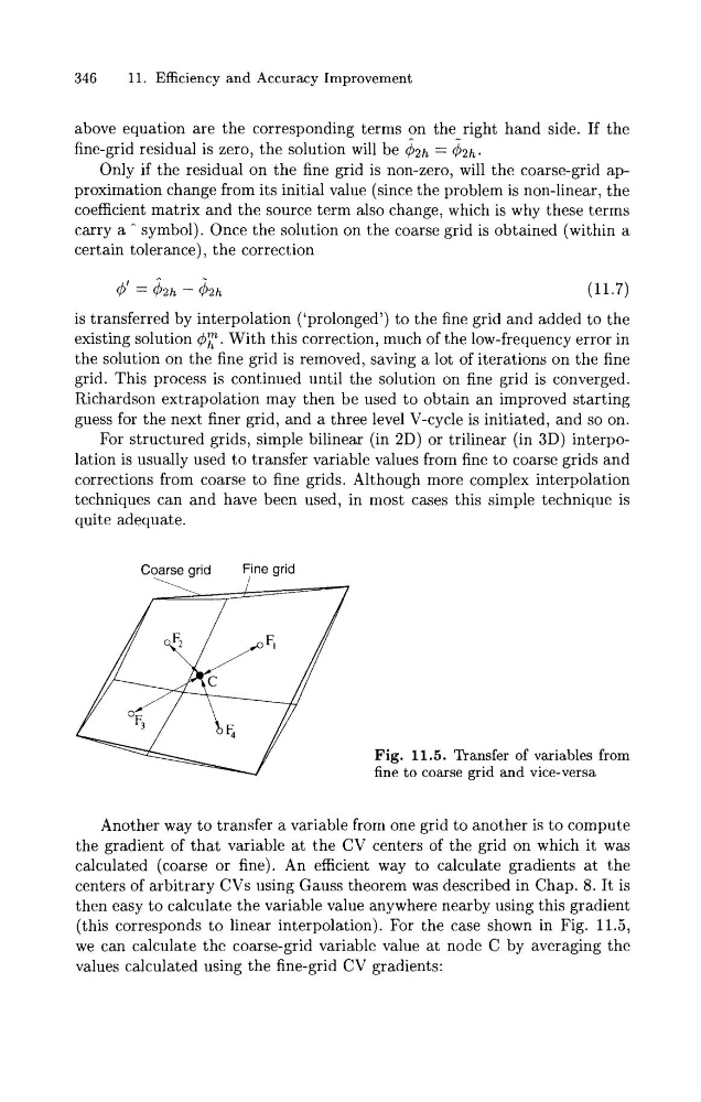
Fig. 11.5. Transfer of variables from
fine to coarse grid and vice-versa
Another way to transfer a variable from one grid to another is to compute
the gradient of that variable at the CV centers of the grid on which it was
calculated (coarse or fine). An efficient way to calculate gradients at the
centers of arbitrary CVs using Gauss theorem was described in Chap. 8. It is
then easy to calculate the variable value anywhere nearby using this gradient
(this corresponds to linear interpolation). For the case shown in Fig. 11.5,
we can calculate the coarse-grid variable value at node C by averaging the
values calculated using the fine-grid CV gradients:
11. Efficiency and Accuracy Improvement
above equation are the corresponding terms on the right hand side. If the
fine-grid residual is zero, the solution will be oh = &h.
Only if the residual on the fine grid is non-zero, will the coarse-grid approximation change from its initial value (since the problem is non-linear, the
coefficient matrix and the source term also change, which is why these terms
carry a A symbol). Once the solution on the coarse grid is obtained (within a
certain tolerance), the correction
is transferred by interpolation ('prolonged') to the fine grid and added to the
existing solution 4 r . With this correction, much of the low-frequency error in
the solution on the fine grid is removed, saving a lot of iterations on the fine
grid. This process is continued until the solution on fine grid is converged.
Richardson extrapolation may then be used to obtain an improved starting
guess for the next finer grid, and a three level V-cycle is initiated, and so on.
For structured grids, simple bilinear (in 2D) or trilinear (in 3D) interpolation is usually used t o transfer variable values from fine to coarse grids and
corrections from coarse to fine grids. Although more complex interpolation
techniques can and have been used, in most cases this simple technique is
quite adequate.
Fig. 11.5. Transfer of variables from
fine to coarse grid and vice-versa
Another way to transfer a variable from one grid to another is to compute
the gradient of that variable at the CV centers of the grid on which it was
calculated (coarse or fine). An efficient way to calculate gradients at the
centers of arbitrary CVs using Gauss theorem was described in Chap. 8. It is
then easy to calculate the variable value anywhere nearby using this gradient
(this corresponds to linear interpolation). For the case shown in Fig. 11.5,
we can calculate the coarse-grid variable value at node C by averaging the
values calculated using the fine-grid CV gradients: