

11.3 Multigrid Methods for Flow Calculation
345
is ideal for solving the Poisson-like pressure or pressure-correction equation
when fractional step or other explicit time-stepping methods are applied to
unsteady flows because accurate solution of the pressure equation is required;
this is often done in LES and DNS of flows in complex geometry. On the other
hand, when implicit methods are used, the linear equations need not be solved
very accurately a t each iteration; reduction of the residual level by one order
of magnitude suffices and can usually be achieved with a few iterations of
one of the basic solvers such as ILU or CG. More accurate solution will not
reduce the number of outer iterations but may increase the computing time.
For steady flow problems, we have seen that implicit solution methods are
preferred and acceleration of the outer iterations is very important. Fortunately, the multigrid method can be applied to outer iterations. The sequence
of operations that constitute one outer iteration is then considered as the
'smoother' in accord with multigrid terminology.
In a multigrid version of a finite volume method for steady flows on a
structured grid, each coarse grid CV is composed of four CVs of the next
finer grid in 2D and eight in 3D. The coarsest grid is usually generated first
and the solution process starts by solving the problem on it. Each CV is then
subdivided in finer CVs. After a converged solution is found on the coarsest
grid, it is interpolated to the next finer grid to provide the starting solution.
Then a two-grid procedure is begun. The process is repeated until the finest
grid is reached and a solution on it is obtained. As noted earlier, this strategy
is called full multigrid procedure (FMG).
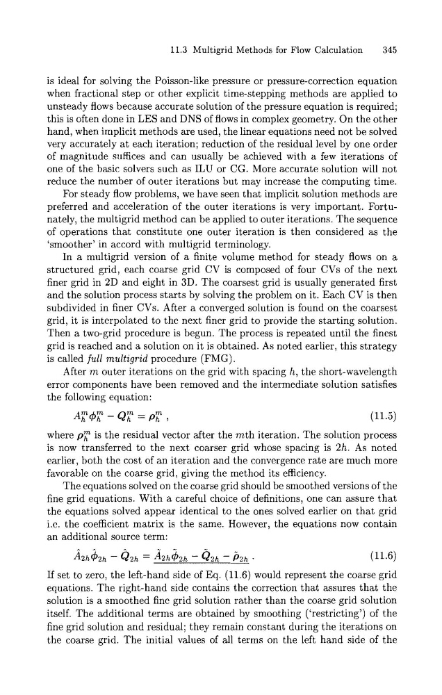
After m outer iterations on the grid with spacing h, the short-wavelength
error components have been removed and the intermediate solution satisfies
the following equation:
where p;lZ is the residual vector after the mth iteration. The solution process
is now transferred to the next coarser grid whose spacing is 2h. As noted
earlier, both the cost of an iteration and the convergence rate are much more
favorable on the coarse grid, giving the method its efficiency.
The equations solved on the coarse grid should be smoothed versions of the
fine grid equations. With a careful choice of definitions, one can assure that
the equations solved appear identical to the ones solved earlier on that grid
i.e. the coefficient matrix is the same. However, the equations now contain
an additional source term:
~ 2 h & ? h
- ~ 2 h
= 132h&h - ~ 2 h
- ~ 2 h
.
(11.6)
If set to zero, the left-hand side of Eq. (11.6) would represent the coarse grid
equations. The right-hand side contains the correction that assures that the
solution is a smoothed fine grid solution rather than the coarse grid solution
itself. The additional terms are obtained by smoothing ('restricting') of the
fine grid solution and residual; they remain constant during the iterations on
the coarse grid. The initial values of all terms on the left hand side of the
345
is ideal for solving the Poisson-like pressure or pressure-correction equation
when fractional step or other explicit time-stepping methods are applied to
unsteady flows because accurate solution of the pressure equation is required;
this is often done in LES and DNS of flows in complex geometry. On the other
hand, when implicit methods are used, the linear equations need not be solved
very accurately a t each iteration; reduction of the residual level by one order
of magnitude suffices and can usually be achieved with a few iterations of
one of the basic solvers such as ILU or CG. More accurate solution will not
reduce the number of outer iterations but may increase the computing time.
For steady flow problems, we have seen that implicit solution methods are
preferred and acceleration of the outer iterations is very important. Fortunately, the multigrid method can be applied to outer iterations. The sequence
of operations that constitute one outer iteration is then considered as the
'smoother' in accord with multigrid terminology.
In a multigrid version of a finite volume method for steady flows on a
structured grid, each coarse grid CV is composed of four CVs of the next
finer grid in 2D and eight in 3D. The coarsest grid is usually generated first
and the solution process starts by solving the problem on it. Each CV is then
subdivided in finer CVs. After a converged solution is found on the coarsest
grid, it is interpolated to the next finer grid to provide the starting solution.
Then a two-grid procedure is begun. The process is repeated until the finest
grid is reached and a solution on it is obtained. As noted earlier, this strategy
is called full multigrid procedure (FMG).
After m outer iterations on the grid with spacing h, the short-wavelength
error components have been removed and the intermediate solution satisfies
the following equation:
where p;lZ is the residual vector after the mth iteration. The solution process
is now transferred to the next coarser grid whose spacing is 2h. As noted
earlier, both the cost of an iteration and the convergence rate are much more
favorable on the coarse grid, giving the method its efficiency.
The equations solved on the coarse grid should be smoothed versions of the
fine grid equations. With a careful choice of definitions, one can assure that
the equations solved appear identical to the ones solved earlier on that grid
i.e. the coefficient matrix is the same. However, the equations now contain
an additional source term:
~ 2 h & ? h
- ~ 2 h
= 132h&h - ~ 2 h
- ~ 2 h
.
(11.6)
If set to zero, the left-hand side of Eq. (11.6) would represent the coarse grid
equations. The right-hand side contains the correction that assures that the
solution is a smoothed fine grid solution rather than the coarse grid solution
itself. The additional terms are obtained by smoothing ('restricting') of the
fine grid solution and residual; they remain constant during the iterations on
the coarse grid. The initial values of all terms on the left hand side of the