

9.4 RANS Models
303
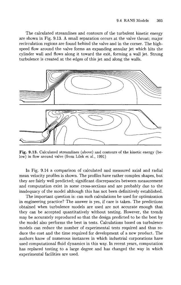
The calculated streamlines and contours of the turbulent kinetic energy
are shown in Fig. 9.13. A small separation occurs at the valve throat; major
recirculation regions are found behind the valve and in the corner. The highspeed flow around the valve forms an expanding annular jet which hits the
cylinder wall and flows along it toward the exit, forming a wall jet. Strong
turbulence is created a t the edges of this jet and along the walls.
Fig. 9.13. Calculated streamlines (above) and contours of the kinetic energy (below) in flow around valve (from Lilek et al., 1991)
In Fig. 9.14 a comparison of calculated and measured axial and radial
mean velocity profiles is shown. The profiles have rather complex shapes, but
they are fairly well predicted; significant discrepancies between measurement
and computation exist in some cross-sections and are probably due to the
inadequacy of the model although this has not been definitively established.
The important question is: can such calculations be used for optimization
in engineering practice? The answer is yes, if care is taken. The predictions
obtained when turbulence models are used are not accurate enough that
they can be accepted quantitatively without testing. However, the trends
may be accurately reproduced so that the design predicted to be the best by
the model also performs the best in tests. Calculations based on turbulence
models can reduce the number of experimental tests required and thus reduce the cost and the time required for development of a new product. The
authors know of numerous instances in which industrial corporations have
used computational fluid dynamics in this way. In recent years, computation
has replaced testing t o a large degree and has changed the way in which
experimental facilities are used.
303
The calculated streamlines and contours of the turbulent kinetic energy
are shown in Fig. 9.13. A small separation occurs at the valve throat; major
recirculation regions are found behind the valve and in the corner. The highspeed flow around the valve forms an expanding annular jet which hits the
cylinder wall and flows along it toward the exit, forming a wall jet. Strong
turbulence is created a t the edges of this jet and along the walls.
Fig. 9.13. Calculated streamlines (above) and contours of the kinetic energy (below) in flow around valve (from Lilek et al., 1991)
In Fig. 9.14 a comparison of calculated and measured axial and radial
mean velocity profiles is shown. The profiles have rather complex shapes, but
they are fairly well predicted; significant discrepancies between measurement
and computation exist in some cross-sections and are probably due to the
inadequacy of the model although this has not been definitively established.
The important question is: can such calculations be used for optimization
in engineering practice? The answer is yes, if care is taken. The predictions
obtained when turbulence models are used are not accurate enough that
they can be accepted quantitatively without testing. However, the trends
may be accurately reproduced so that the design predicted to be the best by
the model also performs the best in tests. Calculations based on turbulence
models can reduce the number of experimental tests required and thus reduce the cost and the time required for development of a new product. The
authors know of numerous instances in which industrial corporations have
used computational fluid dynamics in this way. In recent years, computation
has replaced testing t o a large degree and has changed the way in which
experimental facilities are used.