

302
9. Turbulent Flows
where L is the length scale of the turbulence, usually taken to be L z , k 3 l 2 / ~ .
The introduction of this procedure appears to relieve a great deal of the
difficulty. More details on these and other similar models can be found in a
recent book by Durbin and Pettersson Reif (2001).
9.4.4 Example: Flow Around an Engine Valve
We briefly present an application of the k-E model. Valves in internal combustion engines are usually optimized by performing experiments on steady flows
at several valve lifts. Lilek et al. (1991) reported the results of a combined
numerical and experimental investigation of one particular geometry. The geometry was axi-symmetric, so a 2D solution method using a boundary-fitted
grid was used. Second-order CDS discretization with three systematically
refined grids were used; the finest had 216 x 64 CVs. By comparing the
solutions on these three grids, the discretization error was estimated to be
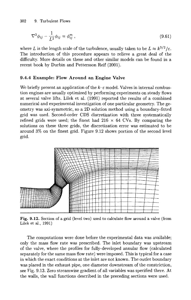
around 3% on the finest grid. Figure 9.12 shows portion of the second level
grid.
Fig. 9.12. Section of a grid (level two) used to calculate flow around a valve (from
Lilek et a]., 1991)
The computations were done before the experimental data was available;
only the mass flow rate was prescribed. The inlet boundary was upstream
of the valve, where the profiles for fully-developed annular flow (calculated
separately for the same mass flow rate) were imposed. This is typical for a case
in which the exact conditions at the inlet are not known. The outlet boundary
was placed in the exhaust pipe, one diameter downstream of the constriction,
see Fig. 9.13. Zero streamwise gradient of all variables was specified there. At
the walls, the wall functions described in the preceding sections were used.
9. Turbulent Flows
where L is the length scale of the turbulence, usually taken to be L z , k 3 l 2 / ~ .
The introduction of this procedure appears to relieve a great deal of the
difficulty. More details on these and other similar models can be found in a
recent book by Durbin and Pettersson Reif (2001).
9.4.4 Example: Flow Around an Engine Valve
We briefly present an application of the k-E model. Valves in internal combustion engines are usually optimized by performing experiments on steady flows
at several valve lifts. Lilek et al. (1991) reported the results of a combined
numerical and experimental investigation of one particular geometry. The geometry was axi-symmetric, so a 2D solution method using a boundary-fitted
grid was used. Second-order CDS discretization with three systematically
refined grids were used; the finest had 216 x 64 CVs. By comparing the
solutions on these three grids, the discretization error was estimated to be
around 3% on the finest grid. Figure 9.12 shows portion of the second level
grid.
Fig. 9.12. Section of a grid (level two) used to calculate flow around a valve (from
Lilek et a]., 1991)
The computations were done before the experimental data was available;
only the mass flow rate was prescribed. The inlet boundary was upstream
of the valve, where the profiles for fully-developed annular flow (calculated
separately for the same mass flow rate) were imposed. This is typical for a case
in which the exact conditions at the inlet are not known. The outlet boundary
was placed in the exhaust pipe, one diameter downstream of the constriction,
see Fig. 9.13. Zero streamwise gradient of all variables was specified there. At
the walls, the wall functions described in the preceding sections were used.