

232
8. Complex Geometries
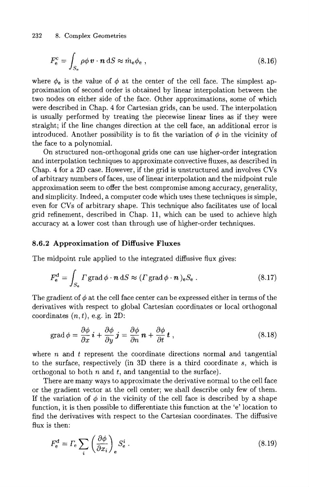
where 4, is the value of 4 a t the center of the cell face. The simplest approximation of second order is obtained by linear interpolation between the
two nodes on either side of the face. Other approximations, some of which
were described in Chap. 4 for Cartesian grids, can be used. The interpolation
is usually performed by treating the piecewise linear lines as if they were
straight; if the line changes direction at the cell face, an additional error is
introduced. Another possibility is to fit the variation of 4 in the vicinity of
the face to a polynomial.
On structured non-orthogonal grids one can use higher-order integration
and interpolation techniques to approximate convective fluxes, as described in
Chap. 4 for a 2D case. However, if the grid is unstructured and involves CVs
of arbitrary numbers of faces, use of linear interpolation and the midpoint rule
approximation seem to offer the best compromise among accuracy, generality,
and simplicity. Indeed, a computer code which uses these techniques is simple,
even for CVs of arbitrary shape. This technique also facilitates use of local
grid refinement, described in Chap. 11, which can be used to achieve high
accuracy a t a lower cost than through use of higher-order techniques.
8.6.2 Approximation of Diffusive Fluxes
The midpoint rule applied to the integrated diffusive flux gives:
The gradient of 4 a t the cell face center can be expressed either in terms of the
derivatives with respect to global Cartesian coordinates or local orthogonal
coordinates (n, t ) , e.g. in 2D:
where n and t represent the coordinate directions normal and tangential
to the surface, respectively (in 3D there is a third coordinate s, which is
orthogonal to both n and t, and tangential to the surface).
There are many ways to approximate the derivative normal to the cell face
or the gradient vector a t the cell center; we shall describe only few of them.
If the variation of 4 in the vicinity of the cell face is described by a shape
function, it is then possible to differentiate this function at the 'e' location t o
find the derivatives with respect to the Cartesian coordinates. The diffusive
flux is then:
8. Complex Geometries
where 4, is the value of 4 a t the center of the cell face. The simplest approximation of second order is obtained by linear interpolation between the
two nodes on either side of the face. Other approximations, some of which
were described in Chap. 4 for Cartesian grids, can be used. The interpolation
is usually performed by treating the piecewise linear lines as if they were
straight; if the line changes direction at the cell face, an additional error is
introduced. Another possibility is to fit the variation of 4 in the vicinity of
the face to a polynomial.
On structured non-orthogonal grids one can use higher-order integration
and interpolation techniques to approximate convective fluxes, as described in
Chap. 4 for a 2D case. However, if the grid is unstructured and involves CVs
of arbitrary numbers of faces, use of linear interpolation and the midpoint rule
approximation seem to offer the best compromise among accuracy, generality,
and simplicity. Indeed, a computer code which uses these techniques is simple,
even for CVs of arbitrary shape. This technique also facilitates use of local
grid refinement, described in Chap. 11, which can be used to achieve high
accuracy a t a lower cost than through use of higher-order techniques.
8.6.2 Approximation of Diffusive Fluxes
The midpoint rule applied to the integrated diffusive flux gives:
The gradient of 4 a t the cell face center can be expressed either in terms of the
derivatives with respect to global Cartesian coordinates or local orthogonal
coordinates (n, t ) , e.g. in 2D:
where n and t represent the coordinate directions normal and tangential
to the surface, respectively (in 3D there is a third coordinate s, which is
orthogonal to both n and t, and tangential to the surface).
There are many ways to approximate the derivative normal to the cell face
or the gradient vector a t the cell center; we shall describe only few of them.
If the variation of 4 in the vicinity of the cell face is described by a shape
function, it is then possible to differentiate this function at the 'e' location t o
find the derivatives with respect to the Cartesian coordinates. The diffusive
flux is then: