

8.6 Finite Volume Methods
233
This is easy t o implement explicitly; an implicit version may be complicated,
depending on the order of the shape function and the number of nodes involved.
Another way to calculate derivatives at the cell face is t o obtain them
first at CV centers, and then interpolate them to the cell faces in the way
4, was. A simple way of doing this is provided by the Gauss' theorem; we
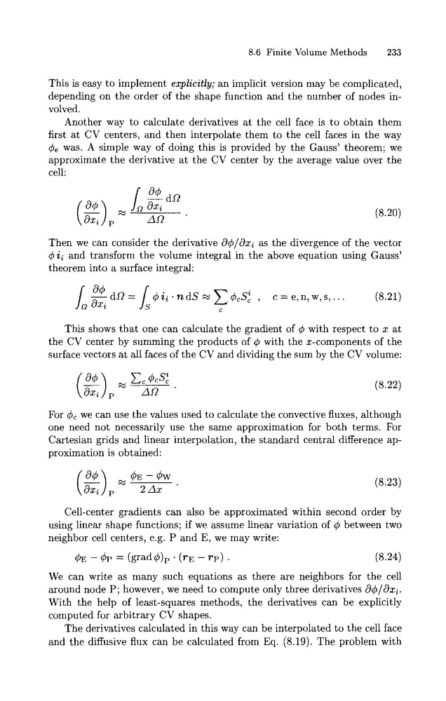
approximate the derivative at the CV center by the average value over the
cell:
Then we can consider the derivative d 4 / d x i as the divergence of the vector
4ii and transform the volume integral in the above equation using Gauss'
theorem into a surface integral:
This shows that one can calculate the gradient of 4 with respect to x at
the CV center by summing the products of 4 with the x-components of the
surface vectors at all faces of the CV and dividing the sum by the CV volume:
For 4, we can use the values used to calculate the convective fluxes, although
one need not necessarily use the same approximation for both terms. For
Cartesian grids and linear interpolation, the standard central difference approximation is obtained:
Cell-center gradients can also be approximated within second order by
using linear shape functions; if we assume linear variation of $ between two
neighbor cell centers, e.g. P and E, we may write:
We can write as many such equations as there are neighbors for the cell
around node P; however, we need to compute only three derivatives d 4 / d x i .
With the help of least-squares methods, the derivatives can be explicitly
computed for arbitrary CV shapes.
The derivatives calculated in this way can be interpolated to the cell face
and the diffusive flux can be calculated from Eq. (8.19). The problem with
233
This is easy t o implement explicitly; an implicit version may be complicated,
depending on the order of the shape function and the number of nodes involved.
Another way to calculate derivatives at the cell face is t o obtain them
first at CV centers, and then interpolate them to the cell faces in the way
4, was. A simple way of doing this is provided by the Gauss' theorem; we
approximate the derivative at the CV center by the average value over the
cell:
Then we can consider the derivative d 4 / d x i as the divergence of the vector
4ii and transform the volume integral in the above equation using Gauss'
theorem into a surface integral:
This shows that one can calculate the gradient of 4 with respect to x at
the CV center by summing the products of 4 with the x-components of the
surface vectors at all faces of the CV and dividing the sum by the CV volume:
For 4, we can use the values used to calculate the convective fluxes, although
one need not necessarily use the same approximation for both terms. For
Cartesian grids and linear interpolation, the standard central difference approximation is obtained:
Cell-center gradients can also be approximated within second order by
using linear shape functions; if we assume linear variation of $ between two
neighbor cell centers, e.g. P and E, we may write:
We can write as many such equations as there are neighbors for the cell
around node P; however, we need to compute only three derivatives d 4 / d x i .
With the help of least-squares methods, the derivatives can be explicitly
computed for arbitrary CV shapes.
The derivatives calculated in this way can be interpolated to the cell face
and the diffusive flux can be calculated from Eq. (8.19). The problem with