

8.6 Finite Volume Methods
231
8.6.1 Approximation of Convective Fluxes
We shall use the midpoint rule approximation of the surface and volume
integrals exclusively. We look first at the calculation of mass fluxes. Only the
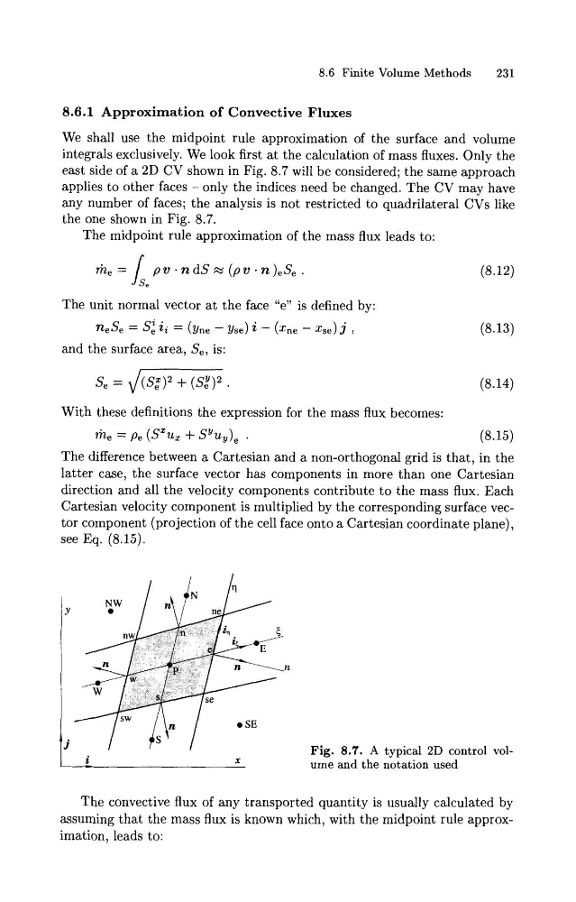
east side of a 2D CV shown in Fig. 8.7 will be considered; the same approach
applies to other faces - only the indices need be changed. The CV may have
any number of faces; the analysis is not restricted to quadrilateral CVs like
the one shown in Fig. 8.7.
The midpoint rule approximation of the mass flux leads to:
r
The unit normal vector a t the face "ex is defined by:
n e S e = S: ii = ( ~ n e - Yse) i - (xne - xse) j ,
(8.13)
and the surface area, S,, is:
With these definitions the expression for the mass flux becomes:
The difference between a Cartesian and a non-orthogonal grid is that, in the
latter case, the surface vector has components in more than one Cartesian
direction and all the velocity components contribute t o the mass flux. Each
Cartesian velocity component is multiplied by the corresponding surface vector component (projection of the cell face onto a Cartesian coordinate plane),
see Eq. (8.15).
Fig. 8.7. A typical 2D control
ume and the notation used
The convective flux of any transported quantity is usually calculated by
assuming that the mass flux is known which, with the midpoint rule approximation, leads to:
231
8.6.1 Approximation of Convective Fluxes
We shall use the midpoint rule approximation of the surface and volume
integrals exclusively. We look first at the calculation of mass fluxes. Only the
east side of a 2D CV shown in Fig. 8.7 will be considered; the same approach
applies to other faces - only the indices need be changed. The CV may have
any number of faces; the analysis is not restricted to quadrilateral CVs like
the one shown in Fig. 8.7.
The midpoint rule approximation of the mass flux leads to:
r
The unit normal vector a t the face "ex is defined by:
n e S e = S: ii = ( ~ n e - Yse) i - (xne - xse) j ,
(8.13)
and the surface area, S,, is:
With these definitions the expression for the mass flux becomes:
The difference between a Cartesian and a non-orthogonal grid is that, in the
latter case, the surface vector has components in more than one Cartesian
direction and all the velocity components contribute t o the mass flux. Each
Cartesian velocity component is multiplied by the corresponding surface vector component (projection of the cell face onto a Cartesian coordinate plane),
see Eq. (8.15).
Fig. 8.7. A typical 2D control
ume and the notation used
The convective flux of any transported quantity is usually calculated by
assuming that the mass flux is known which, with the midpoint rule approximation, leads to: