

148
6. Methods for Unsteady Problems
of being proportional to (AtlAx)'. This term stems from the substitution
(6.41) and is an undesirable feature of the method because the method is
consistent (that is, it yields a solution of the partial differential equation in
the limit of small step sizes) only if At tends faster to zero than Ax.
To obtain higher order accuracy in time, with reasonable limits on stability, a number of authors have used the Adams-Bashforth second and third
order methods and, more commonly, third and fourth order Runge-Kutta
methods.
6.3.2 Implicit Methods
Implicit Euler Method. If stability is a prime requirement, the analysis
of methods for ordinary differential equations suggests use of the backward
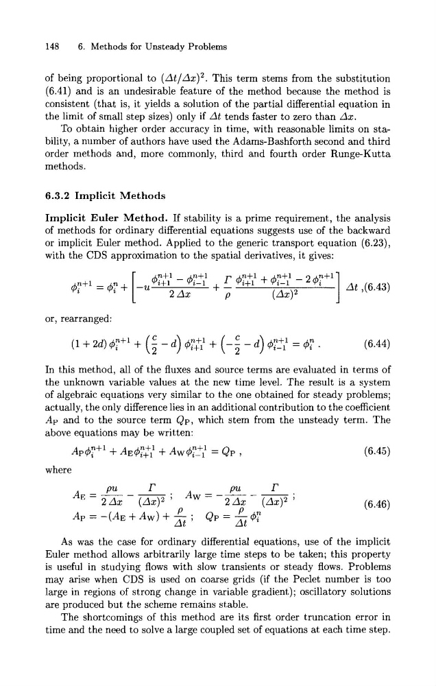
or implicit Euler method. Applied to the generic transport equation (6.23),
with the CDS approximation to the spatial derivatives, it gives:
or, rearranged:
In this method, all of the fluxes and source terms are evaluated in terms of
the unknown variable values a t the new time level. The result is a system
of algebraic equations very similar to the one obtained for steady problems;
actually, the only difference lies in an additional contribution to the coefficient
Ap and to the source term Qp, which stem from the unsteady term. The
above equations may be written:
where
As was the case for ordinary differential equations, use of the implicit
Euler method allows arbitrarily large time steps to be taken; this property
is useful in studying flows with slow transients or steady flows. Problems
may arise when CDS is used on coarse grids (if the Peclet number is too
large in regions of strong change in variable gradient); oscillatory solutions
are produced but the scheme remains stable.
The shortcomings of this method are its first order truncation error in
time and the need to solve a large coupled set of equations at each time step.
6. Methods for Unsteady Problems
of being proportional to (AtlAx)'. This term stems from the substitution
(6.41) and is an undesirable feature of the method because the method is
consistent (that is, it yields a solution of the partial differential equation in
the limit of small step sizes) only if At tends faster to zero than Ax.
To obtain higher order accuracy in time, with reasonable limits on stability, a number of authors have used the Adams-Bashforth second and third
order methods and, more commonly, third and fourth order Runge-Kutta
methods.
6.3.2 Implicit Methods
Implicit Euler Method. If stability is a prime requirement, the analysis
of methods for ordinary differential equations suggests use of the backward
or implicit Euler method. Applied to the generic transport equation (6.23),
with the CDS approximation to the spatial derivatives, it gives:
or, rearranged:
In this method, all of the fluxes and source terms are evaluated in terms of
the unknown variable values a t the new time level. The result is a system
of algebraic equations very similar to the one obtained for steady problems;
actually, the only difference lies in an additional contribution to the coefficient
Ap and to the source term Qp, which stem from the unsteady term. The
above equations may be written:
where
As was the case for ordinary differential equations, use of the implicit
Euler method allows arbitrarily large time steps to be taken; this property
is useful in studying flows with slow transients or steady flows. Problems
may arise when CDS is used on coarse grids (if the Peclet number is too
large in regions of strong change in variable gradient); oscillatory solutions
are produced but the scheme remains stable.
The shortcomings of this method are its first order truncation error in
time and the need to solve a large coupled set of equations at each time step.