

6.3 Application to the Generic Transport Equation
147
This method has first order truncation errors in both space and time and
requires very small step sizes in both variables if errors are to be kept small.
The restriction on the Courant number also has the interpretation that a
fluid particle cannot move more than one grid length in a single time step.
This restriction on the rate of information propagation appears very reasonable but can limit the rate of convergence when methods of this kind are
employed for the solution of steady state problems.
Other explicit schemes may be based on other methods for ordinary differential equations. Indeed, all of the methods described earlier have been
used at one time or another in CFD. A central difference based three time
level method, known as the leapfrog method, will be described next.
Leapfrog Method. A commonly used three-level scheme is the leapfrog
method; it is essentially the application of the midpoint rule integration to a
time interval of size 2At:
4: " = 41-' + f (tn, dn) 2At .
(6.38)
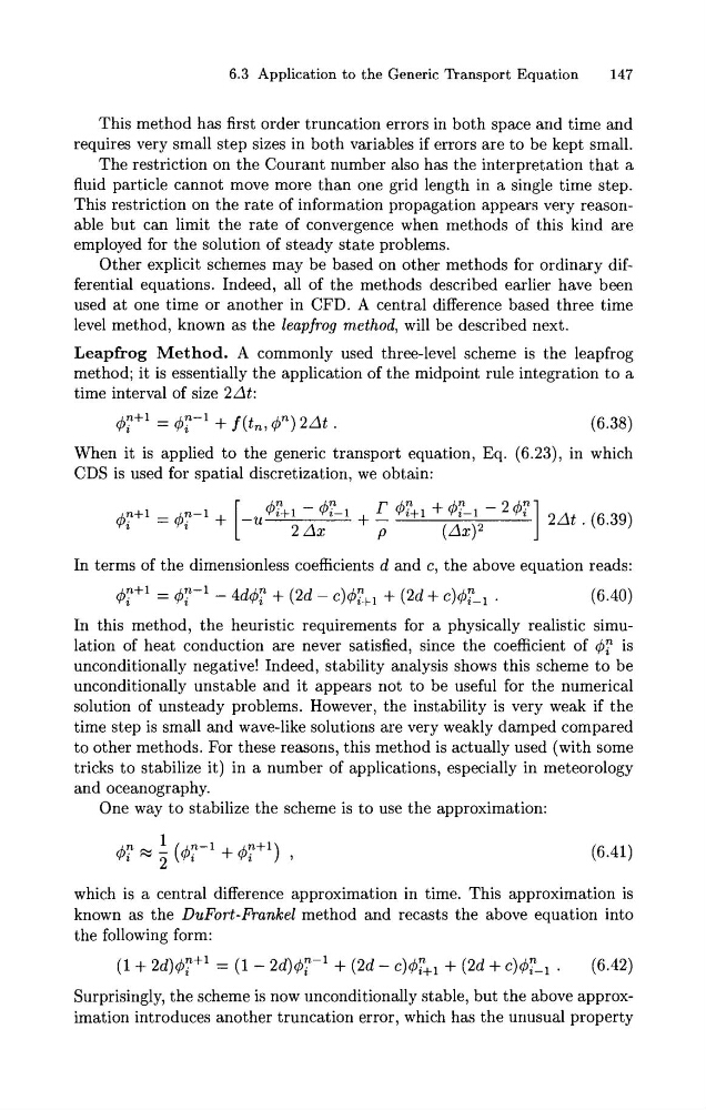
When it is applied to the generic transport equation, Eq. (6.23), in which
CDS is used for spatial discretization, we obtain:
In terms of the dimensionless coefficients d and c, the above equation reads:
In this method, the heuristic requirements for a physically realistic simulation of heat conduction are never satisfied, since the coefficient of 41 is
unconditionally negative! Indeed, stability analysis shows this scheme to be
unconditionally unstable and it appears not to be useful for the numerical
solution of unsteady problems. However, the instability is very weak if the
time step is small and wave-like solutions are very weakly damped compared
to other methods. For these reasons, this method is actually used (with some
tricks to stabilize it) in a number of applications, especially in meteorology
and oceanography.
One way to stabilize the scheme is to use the approximation:
which is a central difference approximation in time. This approximation is
known as the DuFort-Frankel method and recasts the above equation into
the following form:
Surprisingly, the scheme is now unconditionally stable, but the above approximation introduces another truncation error, which has the unusual property
147
This method has first order truncation errors in both space and time and
requires very small step sizes in both variables if errors are to be kept small.
The restriction on the Courant number also has the interpretation that a
fluid particle cannot move more than one grid length in a single time step.
This restriction on the rate of information propagation appears very reasonable but can limit the rate of convergence when methods of this kind are
employed for the solution of steady state problems.
Other explicit schemes may be based on other methods for ordinary differential equations. Indeed, all of the methods described earlier have been
used at one time or another in CFD. A central difference based three time
level method, known as the leapfrog method, will be described next.
Leapfrog Method. A commonly used three-level scheme is the leapfrog
method; it is essentially the application of the midpoint rule integration to a
time interval of size 2At:
4: " = 41-' + f (tn, dn) 2At .
(6.38)
When it is applied to the generic transport equation, Eq. (6.23), in which
CDS is used for spatial discretization, we obtain:
In terms of the dimensionless coefficients d and c, the above equation reads:
In this method, the heuristic requirements for a physically realistic simulation of heat conduction are never satisfied, since the coefficient of 41 is
unconditionally negative! Indeed, stability analysis shows this scheme to be
unconditionally unstable and it appears not to be useful for the numerical
solution of unsteady problems. However, the instability is very weak if the
time step is small and wave-like solutions are very weakly damped compared
to other methods. For these reasons, this method is actually used (with some
tricks to stabilize it) in a number of applications, especially in meteorology
and oceanography.
One way to stabilize the scheme is to use the approximation:
which is a central difference approximation in time. This approximation is
known as the DuFort-Frankel method and recasts the above equation into
the following form:
Surprisingly, the scheme is now unconditionally stable, but the above approximation introduces another truncation error, which has the unusual property