

2.7 Laminar and Thrbulent Flow in Ductti
71
laminar flow
--.
D
-------- ~------------~
turbulent flow
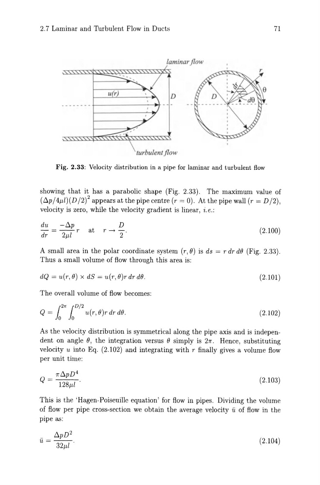
Fig. 2.33: Velocity distribution in a pipe for laminar and turbulent flow
showing that it has a parabolic shape (Fig. 2.33) . The maximum value of
(6.p/4J1l)(D /2)2 appears at the pipe centre (r = 0). At the pipe wall (r = D /2) ,
velocity is zero, while the velocity gradient is linear, i.e.:
du
-6.p
- = - - r
dr
2J1l
at
D
r - > - .
2
(2.100)
A small area in the polar coordinate system (r, e) is ds = r dr de (Fig. 2.33).
Thus a small volume of flow through this area is:
dQ = u(r, e) x dS = u(r, e)r dr de.
(2.101 )
The overall volume of flow becomes:
r27f r D / 2
Q = Jo Jo u(r, e)rdrde .
(2.102)
As the velocity distribution is symmetrical along the pipe axis and is independent on angle e, the integration versus e simply is 27r. Hence, substituting
velocity u into Eq. (2.102) and integrating with r finally gives a volume flow
per unit time:
(2.103)
This is the 'Hagen-Poiseuille equation' for flow in pipes. Dividing the volume
of flow per pipe cross-section we obtain the average velocity u of flow in the
pipe as:
_ 6.pD 2
u = - - .
32J1l
(2.104)
71
laminar flow
--.
D
-------- ~------------~
turbulent flow
Fig. 2.33: Velocity distribution in a pipe for laminar and turbulent flow
showing that it has a parabolic shape (Fig. 2.33) . The maximum value of
(6.p/4J1l)(D /2)2 appears at the pipe centre (r = 0). At the pipe wall (r = D /2) ,
velocity is zero, while the velocity gradient is linear, i.e.:
du
-6.p
- = - - r
dr
2J1l
at
D
r - > - .
2
(2.100)
A small area in the polar coordinate system (r, e) is ds = r dr de (Fig. 2.33).
Thus a small volume of flow through this area is:
dQ = u(r, e) x dS = u(r, e)r dr de.
(2.101 )
The overall volume of flow becomes:
r27f r D / 2
Q = Jo Jo u(r, e)rdrde .
(2.102)
As the velocity distribution is symmetrical along the pipe axis and is independent on angle e, the integration versus e simply is 27r. Hence, substituting
velocity u into Eq. (2.102) and integrating with r finally gives a volume flow
per unit time:
(2.103)
This is the 'Hagen-Poiseuille equation' for flow in pipes. Dividing the volume
of flow per pipe cross-section we obtain the average velocity u of flow in the
pipe as:
_ 6.pD 2
u = - - .
32J1l
(2.104)