

Appendix C Useful Theoretical Approaches and Formulas
487
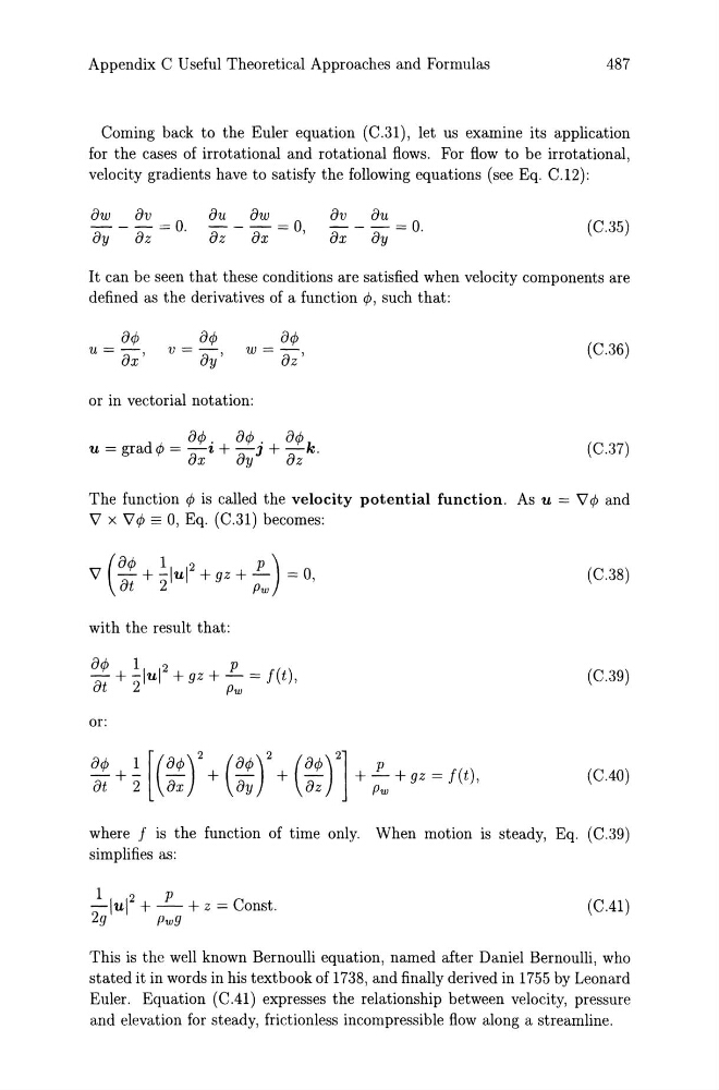
Coming back to the Euler equation (C.3l), let us examine its application
for the cases of irrotational and rotational flows. For flow to be irrotational,
velocity gradients have to satisfy the following equations (see Eq. C.l2):
ow ov
- - -=0.
oy oz
ou ow
- - - = 0
oz ox
'
ov OU
- - - = 0 .
ox oy
(C.35)
It can be seen that these conditions are satisfied when velocity components are
defined as the derivatives of a function o u = -
ox'
o v = oy'
o W = -
oz'
or in vectorial notation:
o u = grad ox oy
oz
(C.36)
(C.37)
The function V x V V - + -lui + gz + - = 0,
( o P )
ot 2
Pw
(C.38)
with the result that:
o P
-+-Iul +gz+-=j(t),
at 2
Pw
(C.39)
or:
o -+- -
+ -
+ -
+-+gz=j(t),
ot 2 ox
oy
oz
Pw
(C.40)
where j is the function of time only. When motion is steady, Eq. (C.39)
simplifies as:
1
2
P
-lui + - + z = Const.
2g
pwg
(C.41)
This is the well known Bernoulli equation, named after Daniel Bernoulli, who
stated it in words in his textbook of 1738, and finally derived in 1755 by Leonard
Euler. Equation (C.4l) expresses the relationship between velocity, pressure
and elevation for steady, frictionless incompressible flow along a streamline.
487
Coming back to the Euler equation (C.3l), let us examine its application
for the cases of irrotational and rotational flows. For flow to be irrotational,
velocity gradients have to satisfy the following equations (see Eq. C.l2):
ow ov
- - -=0.
oy oz
ou ow
- - - = 0
oz ox
'
ov OU
- - - = 0 .
ox oy
(C.35)
It can be seen that these conditions are satisfied when velocity components are
defined as the derivatives of a function o u = -
ox'
o v = oy'
o W = -
oz'
or in vectorial notation:
o u = grad ox oy
oz
(C.36)
(C.37)
The function V x V V - + -lui + gz + - = 0,
( o P )
ot 2
Pw
(C.38)
with the result that:
o P
-+-Iul +gz+-=j(t),
at 2
Pw
(C.39)
or:
o -+- -
+ -
+ -
+-+gz=j(t),
ot 2 ox
oy
oz
Pw
(C.40)
where j is the function of time only. When motion is steady, Eq. (C.39)
simplifies as:
1
2
P
-lui + - + z = Const.
2g
pwg
(C.41)
This is the well known Bernoulli equation, named after Daniel Bernoulli, who
stated it in words in his textbook of 1738, and finally derived in 1755 by Leonard
Euler. Equation (C.4l) expresses the relationship between velocity, pressure
and elevation for steady, frictionless incompressible flow along a streamline.