

15.6 Tidal Mixing and Phytoplankton Production
463
(15.10)
in which depth, h , equals approximately twice of the thickness of the euphotic
zone, and Cnh is the nutrient concentration at depth z = h.
Druet and Zielinski (1994) applied the relationships (15.7)-(15.10) to simulate
the changes of chlorophyll and nutrient concentration for the Baltic Sea conditions. The initial vertical distribution of concentrations cp( z) and cn (z) are
shown in Fig. 15.4a, while Fig. 15.4b illustrates the evolution of these concentrations after 60 min. In the simulation, the level of turbulent mixing intensity
was selected by adopting the velocity shear ou/oz = Const = 0.01 S-l. Thus,
the Richardson number becomes Ri = 10 4 N 2 , where N is the Brunt-Viiisiilii
frequency. Changes in the phytoplankton concentration, cp , are at all times at
the expense of available nutrients.
15.6 Tidal Mixing and Phytoplankton Production
Many highly productive shallow regions of the world's oceans are characterized
by waters which are well mixed all year. The Georges Bank in the Gulf of
Maine, the southern North Sea, the English Channel, and the southern Irish
Sea are examples of such regions. A marked discontinuity in the sea surface
temperature (with a horizontal gradient up to 1°C /km) is observed in these
regions, being a boundary between stratified and vertically mixed regimes.
To support continual mixing of the water column for the full year, energy
sufficient to overcome the barrier of stratification should be supplied to the
system. Following Simpson and Hunter (1974), we estimate the amount of
energy required as the difference between the potential energy of the water
column before and after mixing. When density stratification before mixing has
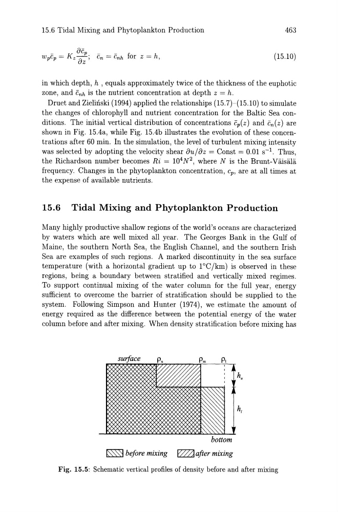
~ before mixing E22ZI after mixing
Fig. 15.5: Schematic vertical profiles of density before and after mixing
463
(15.10)
in which depth, h , equals approximately twice of the thickness of the euphotic
zone, and Cnh is the nutrient concentration at depth z = h.
Druet and Zielinski (1994) applied the relationships (15.7)-(15.10) to simulate
the changes of chlorophyll and nutrient concentration for the Baltic Sea conditions. The initial vertical distribution of concentrations cp( z) and cn (z) are
shown in Fig. 15.4a, while Fig. 15.4b illustrates the evolution of these concentrations after 60 min. In the simulation, the level of turbulent mixing intensity
was selected by adopting the velocity shear ou/oz = Const = 0.01 S-l. Thus,
the Richardson number becomes Ri = 10 4 N 2 , where N is the Brunt-Viiisiilii
frequency. Changes in the phytoplankton concentration, cp , are at all times at
the expense of available nutrients.
15.6 Tidal Mixing and Phytoplankton Production
Many highly productive shallow regions of the world's oceans are characterized
by waters which are well mixed all year. The Georges Bank in the Gulf of
Maine, the southern North Sea, the English Channel, and the southern Irish
Sea are examples of such regions. A marked discontinuity in the sea surface
temperature (with a horizontal gradient up to 1°C /km) is observed in these
regions, being a boundary between stratified and vertically mixed regimes.
To support continual mixing of the water column for the full year, energy
sufficient to overcome the barrier of stratification should be supplied to the
system. Following Simpson and Hunter (1974), we estimate the amount of
energy required as the difference between the potential energy of the water
column before and after mixing. When density stratification before mixing has
~ before mixing E22ZI after mixing
Fig. 15.5: Schematic vertical profiles of density before and after mixing