

8.3 Concentration of Matter for Molecular and Turbulent Diffusion
279
to the fact that the coefficients of turbulent diffusion, Kx and K y , have been
assumed equal to each other.
General Cases of Diffusion. In the scenarios discussed above, relatively
simple environmental conditions have been applied. In particular, coefficients
of turbulent diffusion were assumed to be constant and water depth to be
infinite. However, in many coastal and estuary problems, as well as for more
detailed descriptions of diffusion and mixing phenomena in the deep ocean, a
solution of the full Eq. (8.30) is required. Such a solution can only be achieved
by numerical solution.
In general, two main methods are used. In the first method, the basic system
of equations (for water circulation, and diffusion equation) is solved numerically, using finite difference or finite element techniques in the Eulerian frame of
reference. Examples of applications of such techniques can be found in Fischer
(1981) and Ozmidov (1986). We will return to these techniques in Sect. 8.5,
where mixing processes in estuaries are discussed. The second group are Lagrangian tracking methods, such as the one described in the previous case in
this section. These methods are very flexible and can be applied to threedimensional space as well as allowing for various types of boundary conditions,
such as 'perfectly absorbing surfaces' and reflecting barriers (Csanady, 1973;
Fischer et al., 1979).
Dispersion in Shear Flow Between Parallel Plates and in a Tube. Let
us consider laminar flow between a pair of flat plates separated by a distance
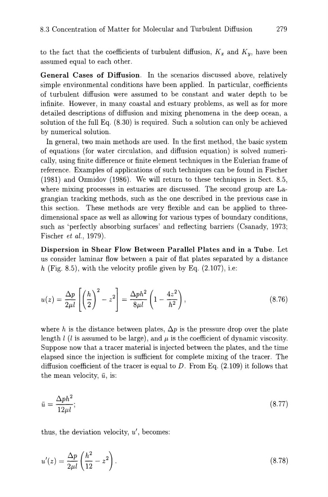
h (Fig. 8.5), with the velocity profile given by Eq. (2.107), i.e:
D"p [(h)2 2] D"ph 2 ( 4z2)
u(z) = 2p,1 ' 2 - z = SiX 1 - h2 '
(8.76)
where h is the distance between plates, D"p is the pressure drop over the plate
length I (I is assumed to be large), and p, is the coefficient of dynamic viscosity.
Suppose now that a tracer material is injected between the plates, and the time
elapsed since the injection is sufficient for complete mixing of the tracer. The
diffusion coefficient of the tracer is equal to D. From Eq. (2.109) it follows that
the mean velocity, u, is:
_ D"ph 2
u = - - '
12p,l '
(8.77)
thus, the deviation velocity, u', becomes:
,
D"p (h2 2)
U (z) = -
- - z .
2p,1 12
(8.78)
279
to the fact that the coefficients of turbulent diffusion, Kx and K y , have been
assumed equal to each other.
General Cases of Diffusion. In the scenarios discussed above, relatively
simple environmental conditions have been applied. In particular, coefficients
of turbulent diffusion were assumed to be constant and water depth to be
infinite. However, in many coastal and estuary problems, as well as for more
detailed descriptions of diffusion and mixing phenomena in the deep ocean, a
solution of the full Eq. (8.30) is required. Such a solution can only be achieved
by numerical solution.
In general, two main methods are used. In the first method, the basic system
of equations (for water circulation, and diffusion equation) is solved numerically, using finite difference or finite element techniques in the Eulerian frame of
reference. Examples of applications of such techniques can be found in Fischer
(1981) and Ozmidov (1986). We will return to these techniques in Sect. 8.5,
where mixing processes in estuaries are discussed. The second group are Lagrangian tracking methods, such as the one described in the previous case in
this section. These methods are very flexible and can be applied to threedimensional space as well as allowing for various types of boundary conditions,
such as 'perfectly absorbing surfaces' and reflecting barriers (Csanady, 1973;
Fischer et al., 1979).
Dispersion in Shear Flow Between Parallel Plates and in a Tube. Let
us consider laminar flow between a pair of flat plates separated by a distance
h (Fig. 8.5), with the velocity profile given by Eq. (2.107), i.e:
D"p [(h)2 2] D"ph 2 ( 4z2)
u(z) = 2p,1 ' 2 - z = SiX 1 - h2 '
(8.76)
where h is the distance between plates, D"p is the pressure drop over the plate
length I (I is assumed to be large), and p, is the coefficient of dynamic viscosity.
Suppose now that a tracer material is injected between the plates, and the time
elapsed since the injection is sufficient for complete mixing of the tracer. The
diffusion coefficient of the tracer is equal to D. From Eq. (2.109) it follows that
the mean velocity, u, is:
_ D"ph 2
u = - - '
12p,l '
(8.77)
thus, the deviation velocity, u', becomes:
,
D"p (h2 2)
U (z) = -
- - z .
2p,1 12
(8.78)