

280
8 Transport in the Oceans and Coastal Zone
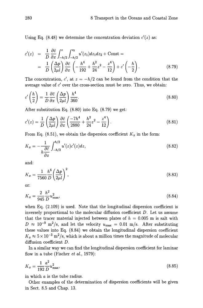
Using Eq. (8.48) we determine the concentration deviation e'(z) as:
e' (z)
1 oe jZ jZ2
- -
u'(zl)dz1dz2 + Const =
D ax -h/2 -h/2
~ (b..p) oe (_~ + h 2 z2 _ z4) + e' (_t:) .
D 2/11 ax 192 24
12
2
(8.79)
The concentration, e', at z = -h/2 can be found from the condition that the
average value of e' over the cross-section must be zero. Thus, we obtain:
e' (%) = ~ ~: (~:Z) 3~~'
After substitution Eq. (8.80) into Eq. (8.79) we get:
From Eq. (8.51), we obtain the dispersion coefficient Kx in the form:
1 jh/2
Kx = -----a= u'(z)e'(z)dz,
h~ -h/2
ax
and:
or:
2 h 2
K = _ _ u 2
x
945 D max'
(8.80)
(8.81 )
(8.82)
(8.83)
(8.84)
when Eq. (2.109) is used. Note that the longitudinal dispersion coefficient is
inversely proportional to the molecular diffusion coefficient D. Let us assume
that the tracer material injected between plates of h = 0.005 m is salt with
D ::::! 10- 9 m 2 /s, and let the velocity Umax = 0.01 m/s. After substituting
these values into Eq. (8.84) we obtain the longitudinal dispersion coefficient
K x ::::! 5 X 10- 3 m 2 /s, which is about a million times the magnitude of molecular
diffusion coefficient D.
In a similar way we can find the longitudinal dispersion coefficient for laminar
flow in a tube (Fischer et al., 1979):
1 a 2
K = _ _ u2
x
192 D max'
in which a is the tube radius.
(8.85)
Other examples of the determination of dispersion coefficients will be given
in Sect. 8.5 and Chap. 13.
8 Transport in the Oceans and Coastal Zone
Using Eq. (8.48) we determine the concentration deviation e'(z) as:
e' (z)
1 oe jZ jZ2
- -
u'(zl)dz1dz2 + Const =
D ax -h/2 -h/2
~ (b..p) oe (_~ + h 2 z2 _ z4) + e' (_t:) .
D 2/11 ax 192 24
12
2
(8.79)
The concentration, e', at z = -h/2 can be found from the condition that the
average value of e' over the cross-section must be zero. Thus, we obtain:
e' (%) = ~ ~: (~:Z) 3~~'
After substitution Eq. (8.80) into Eq. (8.79) we get:
From Eq. (8.51), we obtain the dispersion coefficient Kx in the form:
1 jh/2
Kx = -----a= u'(z)e'(z)dz,
h~ -h/2
ax
and:
or:
2 h 2
K = _ _ u 2
x
945 D max'
(8.80)
(8.81 )
(8.82)
(8.83)
(8.84)
when Eq. (2.109) is used. Note that the longitudinal dispersion coefficient is
inversely proportional to the molecular diffusion coefficient D. Let us assume
that the tracer material injected between plates of h = 0.005 m is salt with
D ::::! 10- 9 m 2 /s, and let the velocity Umax = 0.01 m/s. After substituting
these values into Eq. (8.84) we obtain the longitudinal dispersion coefficient
K x ::::! 5 X 10- 3 m 2 /s, which is about a million times the magnitude of molecular
diffusion coefficient D.
In a similar way we can find the longitudinal dispersion coefficient for laminar
flow in a tube (Fischer et al., 1979):
1 a 2
K = _ _ u2
x
192 D max'
in which a is the tube radius.
(8.85)
Other examples of the determination of dispersion coefficients will be given
in Sect. 8.5 and Chap. 13.