

152
4 How to Determine Wave Parameters
,.-.. 10
CJJ
'" S 9
'-'
~
S 8
E () 7
II)
0..
CJJ
» 6
btl
....
JONSWAP spectrum
II)
Q
5
~
4
3
Pierson-Moskowitz spectrum
2
0.2
0.4
0.6
0.8
1.0
1.2
1.4
1.6
1.8
Frequency (0 (radls)
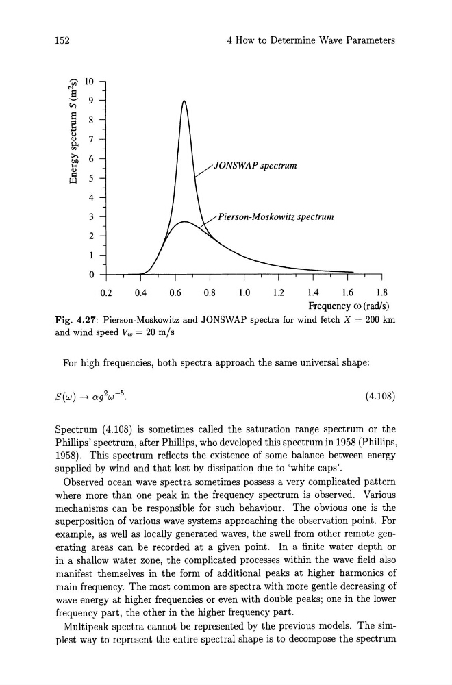
Fig. 4.27: Pierson-Moskowitz and JONSWAP spectra for wind fetch X = 200 km
and wind speed Vw = 20 m/s
For high frequencies, both spectra approach the same universal shape:
(4.108)
Spectrum (4.108) is sometimes called the saturation range spectrum or the
Phillips' spectrum, after Phillips, who developed this spectrum in 1958 (Phillips,
1958). This spectrum reflects the existence of some balance between energy
supplied by wind and that lost by dissipation due to 'white caps'.
Observed ocean wave spectra sometimes possess a very complicated pattern
where more than one peak in the frequency spectrum is observed. Various
mechanisms can be responsible for such behaviour. The obvious one is the
superposition of various wave systems approaching the observation point. For
example, as well as locally generated waves, the swell from other remote generating areas can be recorded at a given point. In a finite water depth or
in a shallow water zone, the complicated processes within the wave field also
manifest themselves in the form of additional peaks at higher harmonics of
main frequency. The most common are spectra with more gentle decreasing of
wave energy at higher frequencies or even with double peaks; one in the lower
frequency part, the other in the higher frequency part.
Multipeak spectra cannot be represented by the previous models. The simplest way to represent the entire spectral shape is to decompose the spectrum
4 How to Determine Wave Parameters
,.-.. 10
CJJ
'" S 9
'-'
~
S 8
E () 7
II)
0..
CJJ
» 6
btl
....
JONSWAP spectrum
II)
Q
5
~
4
3
Pierson-Moskowitz spectrum
2
0.2
0.4
0.6
0.8
1.0
1.2
1.4
1.6
1.8
Frequency (0 (radls)
Fig. 4.27: Pierson-Moskowitz and JONSWAP spectra for wind fetch X = 200 km
and wind speed Vw = 20 m/s
For high frequencies, both spectra approach the same universal shape:
(4.108)
Spectrum (4.108) is sometimes called the saturation range spectrum or the
Phillips' spectrum, after Phillips, who developed this spectrum in 1958 (Phillips,
1958). This spectrum reflects the existence of some balance between energy
supplied by wind and that lost by dissipation due to 'white caps'.
Observed ocean wave spectra sometimes possess a very complicated pattern
where more than one peak in the frequency spectrum is observed. Various
mechanisms can be responsible for such behaviour. The obvious one is the
superposition of various wave systems approaching the observation point. For
example, as well as locally generated waves, the swell from other remote generating areas can be recorded at a given point. In a finite water depth or
in a shallow water zone, the complicated processes within the wave field also
manifest themselves in the form of additional peaks at higher harmonics of
main frequency. The most common are spectra with more gentle decreasing of
wave energy at higher frequencies or even with double peaks; one in the lower
frequency part, the other in the higher frequency part.
Multipeak spectra cannot be represented by the previous models. The simplest way to represent the entire spectral shape is to decompose the spectrum