

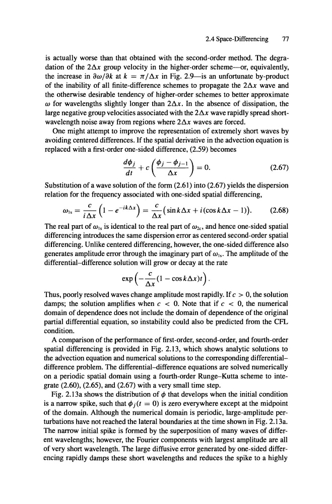
dt
Sx
2.4 Space-Differencing
77
is actually worse than that obtained with the second-order method. The degradation of the 2D.x group velocity in the higher-order scheme-or, equivalently,
the increase in ßw/ßk at k = TC / Sx in Fig. 2.9-is an unfortunate by-product
of the inability of all finite-difference schemes to propagate the 2D.x wave and
the otherwise desirable tendency of higher-order schemes to better approximate
ia for wavelengths slightly longer than 2D.x. In the absence of dissipation, the
large negative group velocities associated with the 2D.x wave rapidly spread shortwavelength noise away from regions where 2D.x waves are forced .
One might attempt to improve the representation of extremely short waves by
avoiding centered differences. If the spatial derivative in the advection equation is
replaced with a first-order one-sided difference, (2.59) becomes
dljJ '
_ J +c (ljJ. J -ljJ' _1)
J
=0.
(2.67)
Substitution of a wave solution of the form (2.61) into (2.67) yields the dispersion
relation for the frequency associated with one-sided spatial differencing,
Wl s =
(1 - eiktU ) =
+ i (cos k D.x - 1)).
(2.68)
lD.X
D.x
The real part of W\ s is identical to the real part of Wz c, and hence one-sided spatial
differencing introduces the same dispersion error as centered second-order spatial
differencing. Unlike centered differencing, however, the one-sided difference also
generates amplitude error through the imaginary part of W\s ' The amplitude of the
differential-difference solution will grow or decay at the rate
exp ( - :x (l - cos kD.X)t) .
Thus, poorly resolved waves change amplitude most rapidly. If c > 0, the solution
damps; the solution amplifies when c < O. Note that if c < 0, the numerical
domain of dependence does not include the domain of dependence of the original
partial differential equation, so instability could also be predicted from the CFL
condition.
A comparison of the performance of first-order, second-order, and fourth-order
spatial differencing is provided in Fig. 2.13, which shows analytic solutions to
the advection equation and numerical solutions to the corresponding differentialdifference problem. The differential-difference equations are solved numerically
on a periodic spatial domain using a fourth-order Runge-Kutta scheme to integrate (2.60), (2.65), and (2.67) with a very sm all time step.
Fig. 2.13a shows the distribution of ljJ that develops when the initial condition
is a narrow spike, such that ljJ jet = 0) is zero everywhere except at the midpoint
of the domain. Although the numerical domain is periodic, large-amplitude perturbations have not reached the lateral boundaries at the time shown in Fig. 2.13a.
The narrow initial spike is formed by the superposition of many waves of different wavelengths; however, the Fourier components with largest amplitude are all
of very short wavelength. The large diffusive error generated by one-sided differencing rapidly damps these short wavelengths and reduces the spike to a highly
Sx
2.4 Space-Differencing
77
is actually worse than that obtained with the second-order method. The degradation of the 2D.x group velocity in the higher-order scheme-or, equivalently,
the increase in ßw/ßk at k = TC / Sx in Fig. 2.9-is an unfortunate by-product
of the inability of all finite-difference schemes to propagate the 2D.x wave and
the otherwise desirable tendency of higher-order schemes to better approximate
ia for wavelengths slightly longer than 2D.x. In the absence of dissipation, the
large negative group velocities associated with the 2D.x wave rapidly spread shortwavelength noise away from regions where 2D.x waves are forced .
One might attempt to improve the representation of extremely short waves by
avoiding centered differences. If the spatial derivative in the advection equation is
replaced with a first-order one-sided difference, (2.59) becomes
dljJ '
_ J +c (ljJ. J -ljJ' _1)
J
=0.
(2.67)
Substitution of a wave solution of the form (2.61) into (2.67) yields the dispersion
relation for the frequency associated with one-sided spatial differencing,
Wl s =
(1 - eiktU ) =
+ i (cos k D.x - 1)).
(2.68)
lD.X
D.x
The real part of W\ s is identical to the real part of Wz c, and hence one-sided spatial
differencing introduces the same dispersion error as centered second-order spatial
differencing. Unlike centered differencing, however, the one-sided difference also
generates amplitude error through the imaginary part of W\s ' The amplitude of the
differential-difference solution will grow or decay at the rate
exp ( - :x (l - cos kD.X)t) .
Thus, poorly resolved waves change amplitude most rapidly. If c > 0, the solution
damps; the solution amplifies when c < O. Note that if c < 0, the numerical
domain of dependence does not include the domain of dependence of the original
partial differential equation, so instability could also be predicted from the CFL
condition.
A comparison of the performance of first-order, second-order, and fourth-order
spatial differencing is provided in Fig. 2.13, which shows analytic solutions to
the advection equation and numerical solutions to the corresponding differentialdifference problem. The differential-difference equations are solved numerically
on a periodic spatial domain using a fourth-order Runge-Kutta scheme to integrate (2.60), (2.65), and (2.67) with a very sm all time step.
Fig. 2.13a shows the distribution of ljJ that develops when the initial condition
is a narrow spike, such that ljJ jet = 0) is zero everywhere except at the midpoint
of the domain. Although the numerical domain is periodic, large-amplitude perturbations have not reached the lateral boundaries at the time shown in Fig. 2.13a.
The narrow initial spike is formed by the superposition of many waves of different wavelengths; however, the Fourier components with largest amplitude are all
of very short wavelength. The large diffusive error generated by one-sided differencing rapidly damps these short wavelengths and reduces the spike to a highly