

60
2. Basic Finite-Difference Methods
1.5
1.0
.-----p
-------lAI
0.5
0.0
, , -
--o
C-------- - ------- --- ---_.
,-- -----0.8
DA
1.2
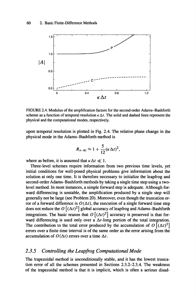
FIGURE 2.4. Modulus of the amplification factors for the second-order Adams-Bashforth
scheme as a funetion of temporal resolution K f!>.t . The solid and dashed lines represent the
physical and the eomputational modes, respectively.
upon temporal resolution is plotted in Fig. 2.4. The relative phase ehange in the
physical mode in the Adams-Bashforth method is
where as before, it is assumed that K ßl « 1.
Three-level schemes require information from two previous time levels, yet
initial conditions for well-posed physical problems give information about the
solution at only one time. It is therefore necessary to initialize the leapfrog and
second-order Adams-Bashforth methods by taking a single time step using a twolevel method. In most instances, a simple forward step is adequate. Although forward differencing is unstable, the amplification produced by a single step will
generally not be large (see Problem 20). Moreover, even though the truncation error of a forward difference is O(ßl), the execution of a single forward time step
does not reduce the 0 [(ßl)2] global accuracy of leapfrog and Adams-Bashforth
integrations. The basic reason that 0 [(ßl)2] accuracy is preserved is that forward differencing is used only over a ßl-10ng portion of the total integration.
The contribution to the total error produced by the accumulation of 0 [(ßl)2]
errors over a finite time interval is of the same order as the error arising from the
accumulation of 0 (ßl) errors over a time ßl .
2.3.5 Controlling the Leapfrog Computational Mode
The trapezoidal method is unconditionally stable, and it has the lowest truncation error of all the schemes presented in Sections 2.3.2-2.3.4. The weakness
of the trapezoidal method is that it is implicit, which is often a serious disad-
2. Basic Finite-Difference Methods
1.5
1.0
.-----p
-------lAI
0.5
0.0
, , -
--o
C-------- - ------- --- ---_.
,-- -----0.8
DA
1.2
FIGURE 2.4. Modulus of the amplification factors for the second-order Adams-Bashforth
scheme as a funetion of temporal resolution K f!>.t . The solid and dashed lines represent the
physical and the eomputational modes, respectively.
upon temporal resolution is plotted in Fig. 2.4. The relative phase ehange in the
physical mode in the Adams-Bashforth method is
where as before, it is assumed that K ßl « 1.
Three-level schemes require information from two previous time levels, yet
initial conditions for well-posed physical problems give information about the
solution at only one time. It is therefore necessary to initialize the leapfrog and
second-order Adams-Bashforth methods by taking a single time step using a twolevel method. In most instances, a simple forward step is adequate. Although forward differencing is unstable, the amplification produced by a single step will
generally not be large (see Problem 20). Moreover, even though the truncation error of a forward difference is O(ßl), the execution of a single forward time step
does not reduce the 0 [(ßl)2] global accuracy of leapfrog and Adams-Bashforth
integrations. The basic reason that 0 [(ßl)2] accuracy is preserved is that forward differencing is used only over a ßl-10ng portion of the total integration.
The contribution to the total error produced by the accumulation of 0 [(ßl)2]
errors over a finite time interval is of the same order as the error arising from the
accumulation of 0 (ßl) errors over a time ßl .
2.3.5 Controlling the Leapfrog Computational Mode
The trapezoidal method is unconditionally stable, and it has the lowest truncation error of all the schemes presented in Sections 2.3.2-2.3.4. The weakness
of the trapezoidal method is that it is implicit, which is often a serious disad-