

2.3 Time-Differencing
61
vantage in computing numerical solutions to wave propagation problems. The
best explicit scheme presented in the preceding sections might appear to be the
leapfrog scheme . The leapfrog scheme is stable (unlike the second-order RungeKutta and Adams-Bashforth methods), it is of second order (unlike the Matsuno
method), and it requires only one function evaluation per time step (unlike the
Matsuno and Runge-Kutta schemes) . The weakness of the leapfrog scheme is
its undamped computational mode, which slowly amplifies during simulations of
nonlinear wave propagation problems and generates an instability often known as
"time splitting ,"
One way to control the growth of the computational mode is to periodically
discard the data from the n - I time level (or altematively, to average the n and
n - I time-level solutions) and to restart the integration using a two-time-level
method. Forward differencing is often used to reinitialize leapfrog integrations.
Forward differencing is easy to implement, but since it is a first-order scheme, it
degrades the second-order accuracy of the unadulterated leapfrog method. In addition, forward differencing is unstable and tends to amplify the high-frequency
components of the solution. Moreover, it is difficult to quantify these adverse effects, since they vary according to the number of leapfrog steps between each
forward step. Restarting with a second-order Runge-Kutta scheme is a far OOtter choice, since this preserves second-order accuracy and produces less unstable
amplification. The midpoint method is one second-order Runge-Kutta formulation that can be used to restart leapfrog integrations in complex numerical models
without greatly complicating the model code. A midpoint-method restart may
be implemented by taking a forward step of length l:!..t /2 followed by a single
leapfrog step of length !:!..t /2.
In atmospheric science , it is common, though questionable, practice to control
the computational mode through the use of a second-order time filter. Consider,
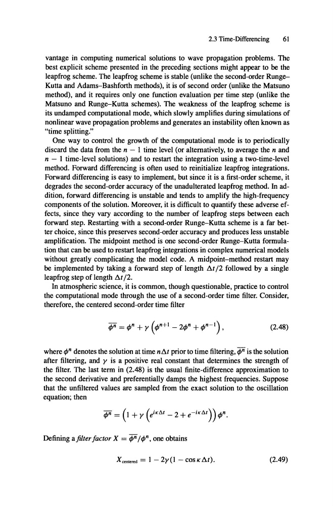
therefore, the centered second-order time filter
(2.48)
where rP n denotes the solution at time n S: prior to time filtering, rP n is the solution
after filtering, and y is a positive real constant that determines the strength of
the filter. The last term in (2.48) is the usual finite-difference approximation to
the second derivative and preferentially damps the highest frequencies. Suppose
that the unfiltered values are sampled from the exact solution to the oscillation
equation; then
Defining afi/ter factor X = rP n /rPn , one obtains
X cenlered = I - 2y(l - COSK!:!..t).
(2.49)
61
vantage in computing numerical solutions to wave propagation problems. The
best explicit scheme presented in the preceding sections might appear to be the
leapfrog scheme . The leapfrog scheme is stable (unlike the second-order RungeKutta and Adams-Bashforth methods), it is of second order (unlike the Matsuno
method), and it requires only one function evaluation per time step (unlike the
Matsuno and Runge-Kutta schemes) . The weakness of the leapfrog scheme is
its undamped computational mode, which slowly amplifies during simulations of
nonlinear wave propagation problems and generates an instability often known as
"time splitting ,"
One way to control the growth of the computational mode is to periodically
discard the data from the n - I time level (or altematively, to average the n and
n - I time-level solutions) and to restart the integration using a two-time-level
method. Forward differencing is often used to reinitialize leapfrog integrations.
Forward differencing is easy to implement, but since it is a first-order scheme, it
degrades the second-order accuracy of the unadulterated leapfrog method. In addition, forward differencing is unstable and tends to amplify the high-frequency
components of the solution. Moreover, it is difficult to quantify these adverse effects, since they vary according to the number of leapfrog steps between each
forward step. Restarting with a second-order Runge-Kutta scheme is a far OOtter choice, since this preserves second-order accuracy and produces less unstable
amplification. The midpoint method is one second-order Runge-Kutta formulation that can be used to restart leapfrog integrations in complex numerical models
without greatly complicating the model code. A midpoint-method restart may
be implemented by taking a forward step of length l:!..t /2 followed by a single
leapfrog step of length !:!..t /2.
In atmospheric science , it is common, though questionable, practice to control
the computational mode through the use of a second-order time filter. Consider,
therefore, the centered second-order time filter
(2.48)
where rP n denotes the solution at time n S: prior to time filtering, rP n is the solution
after filtering, and y is a positive real constant that determines the strength of
the filter. The last term in (2.48) is the usual finite-difference approximation to
the second derivative and preferentially damps the highest frequencies. Suppose
that the unfiltered values are sampled from the exact solution to the oscillation
equation; then
Defining afi/ter factor X = rP n /rPn , one obtains
X cenlered = I - 2y(l - COSK!:!..t).
(2.49)