

2.3 Time-Differencing
59
The computational mode and the physical mode oscillate in opposite directions.
In the limit of good time resolution,
(KI:1t)2
R+leapfrog
1 + --6-'
showing that leapfrog time differencing is accelerating.
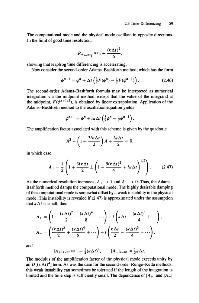
Now consider the second-order Adams-Bashforth method, which has the form
(2.46)
The second-order Adams-Bashforth formula may be interpreted as numerical
integration via the midpoint method, except that the value of the integrand at
the midpoint, F(ifJn+I /2), is obtained by linear extrapolation. Application of the
Adams-Bashforth method to the oscillation equation yields
ifJn+1 = ifJn + iKI:1t OifJ n _1ifJn-I) .
The amplification factor associated with this scheme is given by the quadratic
A 2 _ (I +
A + iK:t = 0,
in which case
I
3iK I:1t
9(KI:1t)2
1 /2 )
A± = 2 (
2± ( I - 4 + iKl:1t ) . (2.47)
As the numerical resolution increases, A+
land A_
O. Thus, the AdamsBashforth method damps the computational mode. The highly desirable damping
of the computational mode is somewhat offset by a weak instability in the physical
mode . This instability is revealed if (2.47) is approximated under the assumption
that KI:1t is smalI; then
A+ = (I _
_
_ . . -) + i (Kl:1t +
+ .. -),
A_ = (K I:1t)2 + (K1:1t)4 + . . .) + i (K I:1t _ (KI:1t)3 _ .. .)
2
8
2
4
'
and
IA+IA-B2 I + !(KI:1t)4,
IA_IA-B2 1Kl:1t.
The modulus of the amplification factor of the physical mode exceeds unity by
an O[(K I:1t)4] term. As was the case for the second-order Runge-Kutta methods,
this weak instability can sometimes be tolerated if the length of the integration is
limited and the time step is sufficiently smalI. The dependence of IA+I and lA_I
59
The computational mode and the physical mode oscillate in opposite directions.
In the limit of good time resolution,
(KI:1t)2
R+leapfrog
1 + --6-'
showing that leapfrog time differencing is accelerating.
Now consider the second-order Adams-Bashforth method, which has the form
(2.46)
The second-order Adams-Bashforth formula may be interpreted as numerical
integration via the midpoint method, except that the value of the integrand at
the midpoint, F(ifJn+I /2), is obtained by linear extrapolation. Application of the
Adams-Bashforth method to the oscillation equation yields
ifJn+1 = ifJn + iKI:1t OifJ n _1ifJn-I) .
The amplification factor associated with this scheme is given by the quadratic
A 2 _ (I +
A + iK:t = 0,
in which case
I
3iK I:1t
9(KI:1t)2
1 /2 )
A± = 2 (
2± ( I - 4 + iKl:1t ) . (2.47)
As the numerical resolution increases, A+
land A_
O. Thus, the AdamsBashforth method damps the computational mode. The highly desirable damping
of the computational mode is somewhat offset by a weak instability in the physical
mode . This instability is revealed if (2.47) is approximated under the assumption
that KI:1t is smalI; then
A+ = (I _
_
_ . . -) + i (Kl:1t +
+ .. -),
A_ = (K I:1t)2 + (K1:1t)4 + . . .) + i (K I:1t _ (KI:1t)3 _ .. .)
2
8
2
4
'
and
IA+IA-B2 I + !(KI:1t)4,
IA_IA-B2 1Kl:1t.
The modulus of the amplification factor of the physical mode exceeds unity by
an O[(K I:1t)4] term. As was the case for the second-order Runge-Kutta methods,
this weak instability can sometimes be tolerated if the length of the integration is
limited and the time step is sufficiently smalI. The dependence of IA+I and lA_I