

7.3 Fractional-Step Methods
363
· 10
2.5
(a)
!
,..... P
E
..>(
......,
x (km)
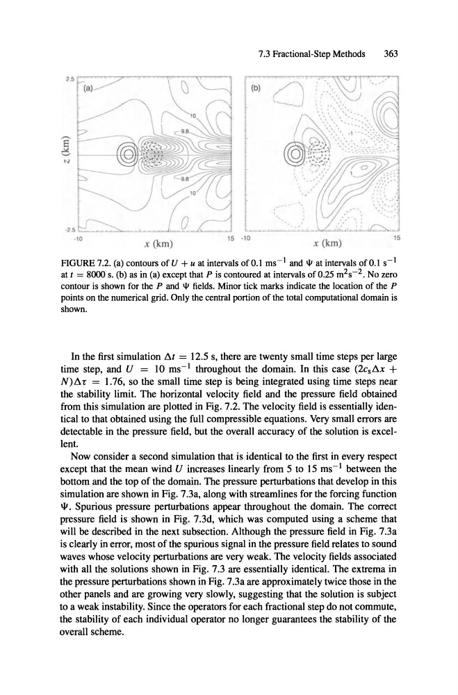
FIGURE7.2. (a) contours of U + u at intervals of 0.1 ms-) and l\J at intervals of 0.1 s-)
at 1 = 8000 s. (b) as in (a) except that P is contoured at intervals of 0.25 m 2s-2 . No zero
contour is shown for the P and l\J tields. Minor tick marks indicate the location of the P
points on the numerical grid. Only the central portionof the total computational domainis
shown.
In the first simulation ßI = 12.5 s, there are twenty small time steps per large
time step, and U = 10 ms"! throughout the domain. In this case (2c sßx +
N)ßr = 1.76, so the small time step is being integrated using time steps near
the stability limit. The horizontal velocity field and the press ure field obtained
from this simulation are plotted in Fig. 7.2. The velocity field is essentially identical to that obtained using the full compressible equations. Very small errors are
detectable in the press ure field, but the overall accuracy of the solution is excellent.
Now consider a second simulation that is identical to the first in every respect
except that the mean wind U increases linearly from 5 to 15 ms-) between the
bottom and the top of the domain . The pressure perturbations that develop in this
simulation are shown in Fig. 7.3a, along with streamlines for the forcing function
\IJ . Spurious pressure perturbations appear throughout the doma in. The correct
pressure field is shown in Fig. 7.3d, which was computed using a scheme that
will be described in the next subsection. Although the pressure field in Fig. 7.3a
is clearly in error, most of the spurious signal in the pressure field relates to sound
waves whose velocity perturbations are very weak . The velocity fields associated
with all the solutions shown in Fig. 7.3 are essentially identical. The extrema in
the pressure perturbations shown in Fig. 7.3a are approximately twice those in the
other panels and are growing very slowly, suggesting that the solution is subject
to a weak instability. Since the operators for each fractional step do not commute,
the stability of each individual operator no longer guarantees the stability of the
overall scheme.
363
· 10
2.5
(a)
!
,..... P
E
..>(
......,
x (km)
FIGURE7.2. (a) contours of U + u at intervals of 0.1 ms-) and l\J at intervals of 0.1 s-)
at 1 = 8000 s. (b) as in (a) except that P is contoured at intervals of 0.25 m 2s-2 . No zero
contour is shown for the P and l\J tields. Minor tick marks indicate the location of the P
points on the numerical grid. Only the central portionof the total computational domainis
shown.
In the first simulation ßI = 12.5 s, there are twenty small time steps per large
time step, and U = 10 ms"! throughout the domain. In this case (2c sßx +
N)ßr = 1.76, so the small time step is being integrated using time steps near
the stability limit. The horizontal velocity field and the press ure field obtained
from this simulation are plotted in Fig. 7.2. The velocity field is essentially identical to that obtained using the full compressible equations. Very small errors are
detectable in the press ure field, but the overall accuracy of the solution is excellent.
Now consider a second simulation that is identical to the first in every respect
except that the mean wind U increases linearly from 5 to 15 ms-) between the
bottom and the top of the domain . The pressure perturbations that develop in this
simulation are shown in Fig. 7.3a, along with streamlines for the forcing function
\IJ . Spurious pressure perturbations appear throughout the doma in. The correct
pressure field is shown in Fig. 7.3d, which was computed using a scheme that
will be described in the next subsection. Although the pressure field in Fig. 7.3a
is clearly in error, most of the spurious signal in the pressure field relates to sound
waves whose velocity perturbations are very weak . The velocity fields associated
with all the solutions shown in Fig. 7.3 are essentially identical. The extrema in
the pressure perturbations shown in Fig. 7.3a are approximately twice those in the
other panels and are growing very slowly, suggesting that the solution is subject
to a weak instability. Since the operators for each fractional step do not commute,
the stability of each individual operator no longer guarantees the stability of the
overall scheme.