

6.2 Forcing in the Lagrangian Frame
315
o
-1.0
_.1.-- ,
...........:r:::,
!
\ .,\
:
;
2
........
............
o
1.0
o
- 1
o
-1.0
1.0
2
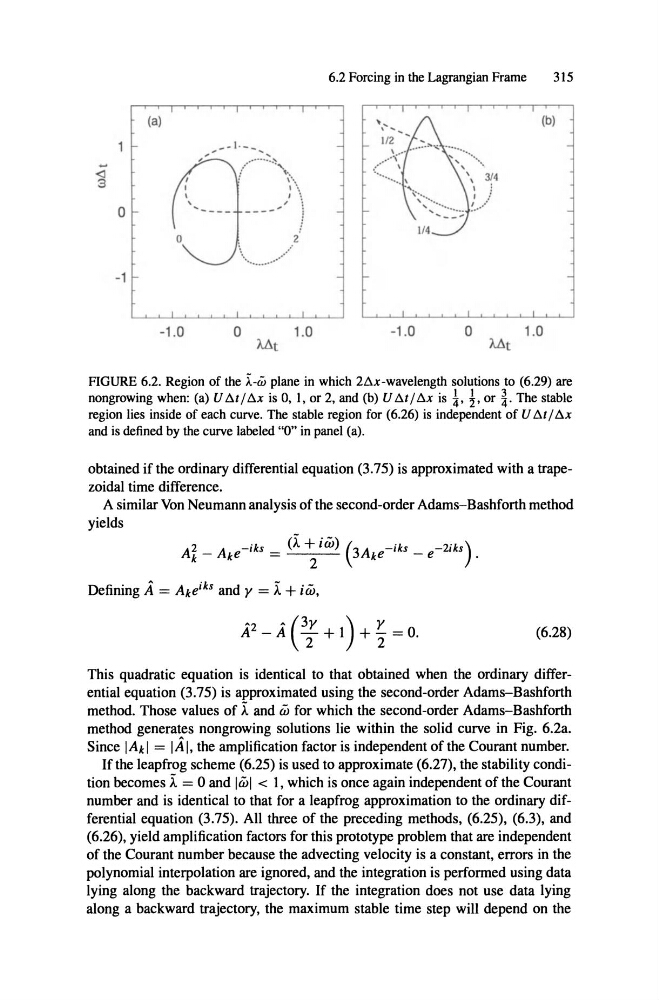
FIGURE 6.2. Region of the X-w plane in which 2Äx-wavelength solutions to (6.29) are
nongrowing when: (a) U Ät / Äx is 0, I, or 2, and (b) U Ät / Äx is i, i,or The stable
region lies inside of each curve. The stable region for (6.26) is independent of U Ät / Äx
and is defined by the curve labeled"0" in panel (a).
obtained if the ordinary differential equation (3.75) is approximated with a trape -
zoidal time difference.
A similar Von Neumann analysis of the second-order Adams-Bashforth method
yields
A 2 k - A ke - iks = (i + iiiJ) (3A ke - iks - e -2ikS) .
Defining A= Ake iks and y = i + iiiJ,
2
A - AC; + I) + i = o.
(6.28)
This quadratic equation is identical to that obtained when the ordinary differential equation (3.75) is approx imated using the second-order Adams-Bashforth
method. Those values of i and iiJ for which the second-order Adams-Bashforth
method generates nongrowing solutions lie within the solid curve in Fig. 6.2a.
Since IAk I = IAI,the amplification factor is independent of the Courant number.
If the leapfrog scheme (6.25) is used to approximate (6.27), the stability condition becomes i = 0 and liiJl < I, which is once again independent of the Courant
number and is identical to that for a leapfrog approximation to the ordinary differential equation (3.75). All three of the preceding methods, (6.25), (6.3), and
(6.26), yield amplification factors for this prototype problem that are independent
of the Courant number because the advecting velocity is a constant, errors in the
polynomial interpolation are ignored, and the integration is performed using data
Iying along the backward trajectory. If the integration does not use data lying
along a backward trajectory, the maximum stable time step will depend on the
315
o
-1.0
_.1.-- ,
...........:r:::,
!
\ .,\
:
;
2
........
............
o
1.0
o
- 1
o
-1.0
1.0
2
FIGURE 6.2. Region of the X-w plane in which 2Äx-wavelength solutions to (6.29) are
nongrowing when: (a) U Ät / Äx is 0, I, or 2, and (b) U Ät / Äx is i, i,or The stable
region lies inside of each curve. The stable region for (6.26) is independent of U Ät / Äx
and is defined by the curve labeled"0" in panel (a).
obtained if the ordinary differential equation (3.75) is approximated with a trape -
zoidal time difference.
A similar Von Neumann analysis of the second-order Adams-Bashforth method
yields
A 2 k - A ke - iks = (i + iiiJ) (3A ke - iks - e -2ikS) .
Defining A= Ake iks and y = i + iiiJ,
2
A - AC; + I) + i = o.
(6.28)
This quadratic equation is identical to that obtained when the ordinary differential equation (3.75) is approx imated using the second-order Adams-Bashforth
method. Those values of i and iiJ for which the second-order Adams-Bashforth
method generates nongrowing solutions lie within the solid curve in Fig. 6.2a.
Since IAk I = IAI,the amplification factor is independent of the Courant number.
If the leapfrog scheme (6.25) is used to approximate (6.27), the stability condition becomes i = 0 and liiJl < I, which is once again independent of the Courant
number and is identical to that for a leapfrog approximation to the ordinary differential equation (3.75). All three of the preceding methods, (6.25), (6.3), and
(6.26), yield amplification factors for this prototype problem that are independent
of the Courant number because the advecting velocity is a constant, errors in the
polynomial interpolation are ignored, and the integration is performed using data
Iying along the backward trajectory. If the integration does not use data lying
along a backward trajectory, the maximum stable time step will depend on the