

4.5 The Finite-Element Method
233
y
L -
X
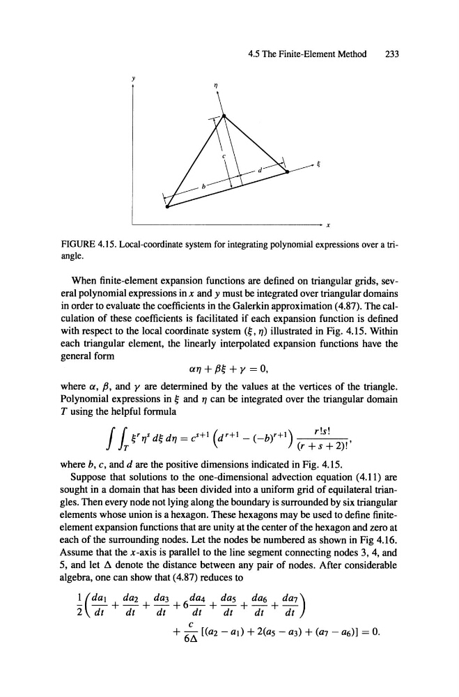
FIGURE 4.15. Local-coordinate system for integrating polynomial expressions over a triangle.
When finite-elernent expansion functions are defined on triangular grids, several polynomial expressions in x and y must be integrated over triangular domains
in order to evaluate the coefficients in the Galerkin approximation (4.87). The calculation of these coefficients is facilitated if each expansion function is defined
with respect to the local coordinate system
TJ) illustrated in Fig. 4.15. Within
each triangular element, the linearly interpolated expansion functions have the
general form
IXTJ + + y = 0,
where IX, ß, and y are determined by the values at the vertices of the triangle.
Polynomial expressions in and TJ can be integrated over the triangular domain
T using the helpful formula
f [
lr
dTJ = c S + 1 (d r+1 _ (_b)r+l)
r!s!
(r +s + 2)!
,
where b, c, and d are the positive dimensions indicated in Fig. 4.15.
Suppose that solutions to the one-dimensional advection equation (4.11) are
sought in a domain that has been divided into a uniform grid of equilateral triangles. Then every node not lying along the boundary is surrounded by six triangular
elements whose union is a hexagon. These hexagons may be used to define finiteelement expansion functions that are unity at the center of the hexagon and zero at
each of the surrounding nodes. Let the nodes be numbered as shown in Fig 4.16.
Assume that the x-axis is parallel to the line segment connecting nodes 3, 4, and
5, and let /i. denote the distance between any pair of nodes. After considerable
algebra, one can show that (4.87) reduces to
1 (da l
daz
da3
6da4
das
da6
da7)
2 dt + dt + dt + dt + dt + dt + dt
233
y
L -
X
FIGURE 4.15. Local-coordinate system for integrating polynomial expressions over a triangle.
When finite-elernent expansion functions are defined on triangular grids, several polynomial expressions in x and y must be integrated over triangular domains
in order to evaluate the coefficients in the Galerkin approximation (4.87). The calculation of these coefficients is facilitated if each expansion function is defined
with respect to the local coordinate system
TJ) illustrated in Fig. 4.15. Within
each triangular element, the linearly interpolated expansion functions have the
general form
IXTJ + + y = 0,
where IX, ß, and y are determined by the values at the vertices of the triangle.
Polynomial expressions in and TJ can be integrated over the triangular domain
T using the helpful formula
f [
lr
dTJ = c S + 1 (d r+1 _ (_b)r+l)
r!s!
(r +s + 2)!
,
where b, c, and d are the positive dimensions indicated in Fig. 4.15.
Suppose that solutions to the one-dimensional advection equation (4.11) are
sought in a domain that has been divided into a uniform grid of equilateral triangles. Then every node not lying along the boundary is surrounded by six triangular
elements whose union is a hexagon. These hexagons may be used to define finiteelement expansion functions that are unity at the center of the hexagon and zero at
each of the surrounding nodes. Let the nodes be numbered as shown in Fig 4.16.
Assume that the x-axis is parallel to the line segment connecting nodes 3, 4, and
5, and let /i. denote the distance between any pair of nodes. After considerable
algebra, one can show that (4.87) reduces to
1 (da l
daz
da3
6da4
das
da6
da7)
2 dt + dt + dt + dt + dt + dt + dt