

,
232
4. Series-Expansion Methods
is approximated using the pagoda-function finite-element method, evaluation of
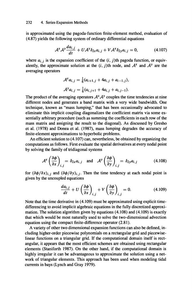
(4.87) yields the following system of ordinary differential equations
A XAy - dt '- + U
dai j
AY 82 a, . + V
x I,}
A X 82 ai . = 0
Y I,}
(4.107)
where ai,j is the expansion coefficient of the (i, j)th pagoda function , or equivalently, the approximate solution at the (i, j)th node, and AX and AY are the
averaging operators
AYa· . = l(a ' '+ 1 + 4a . . + a' '- 1) .
I ,}
6 I ,}
I ,}
I ,}
The product of the averaging operators AX AY couples the time tendencies at nine
different nodes and generates a band matrix with a very wide bandwidth. One
technique, known as "mass lumping,' that has been occasionally advocated to
eliminate this implicit coupling diagonalizes the coefficient matrix via some essentially arbitrary procedure (such as summing the coefficients in each row of the
mass matrix and assigning the result to the diagonal). As discussed by Gresho
et al. (1978) and Donea et al. (1987), mass lumping degrades the accuracy of
finite-element approximations to hyperbolic problems.
An efficient solution to (4.107) can, nevertheless, be obtained by organizing the
computations as folIows. First evaluate the spatial derivatives at every nodal point
by solving the family of tridiagonal systems
and
ifJ)
AY (a ay . . = 82 y a, .
I ,}
I,}
a I ,}
A
X
(a ifJ) =
X
. .
82 a, .
x I ,}
(4.108)
for (aifJ/aX)i, j and (aifJ/aY)i,j . Then the time tendency at each nodal point is
given by the uncoupled equations
dai,j + U (a ifJ)
dt
ax . .
I ,)
+ V (a ifJ)
ay ..
= O.
I ,}
(4.109)
Note that the time derivative in (4.109) must be approximated using explicit timedifferencing to avoid implicit algebraic equations in the fully discretized approximation. The solution algorithm given by equations (4.108) and (4.109) is exactly
that which would be most naturally used to solve the two-dimensional advection
equation using the compact finite-difference operator (2.81) ,
A variety of other two dimensional expansion functions can also be defined, including higher-order piecewise polynomials on a reetangular grid and piecewiselinear functions on a triangular grid. If the computational domain itself is rectangular, it appears that the most efficient schemes are obtained using reetangular
elements (Staniforth 1987), On the other hand, if the computational domain is
highly irregular it can be advantageous to approximate the solution using a network of triangular elements. This approach has been used when modeling tidal
currents in bays (Lynch and Gray 1979).
232
4. Series-Expansion Methods
is approximated using the pagoda-function finite-element method, evaluation of
(4.87) yields the following system of ordinary differential equations
A XAy - dt '- + U
dai j
AY 82 a, . + V
x I,}
A X 82 ai . = 0
Y I,}
(4.107)
where ai,j is the expansion coefficient of the (i, j)th pagoda function , or equivalently, the approximate solution at the (i, j)th node, and AX and AY are the
averaging operators
AYa· . = l(a ' '+ 1 + 4a . . + a' '- 1) .
I ,}
6 I ,}
I ,}
I ,}
The product of the averaging operators AX AY couples the time tendencies at nine
different nodes and generates a band matrix with a very wide bandwidth. One
technique, known as "mass lumping,' that has been occasionally advocated to
eliminate this implicit coupling diagonalizes the coefficient matrix via some essentially arbitrary procedure (such as summing the coefficients in each row of the
mass matrix and assigning the result to the diagonal). As discussed by Gresho
et al. (1978) and Donea et al. (1987), mass lumping degrades the accuracy of
finite-element approximations to hyperbolic problems.
An efficient solution to (4.107) can, nevertheless, be obtained by organizing the
computations as folIows. First evaluate the spatial derivatives at every nodal point
by solving the family of tridiagonal systems
and
ifJ)
AY (a ay . . = 82 y a, .
I ,}
I,}
a I ,}
A
X
(a ifJ) =
X
. .
82 a, .
x I ,}
(4.108)
for (aifJ/aX)i, j and (aifJ/aY)i,j . Then the time tendency at each nodal point is
given by the uncoupled equations
dai,j + U (a ifJ)
dt
ax . .
I ,)
+ V (a ifJ)
ay ..
= O.
I ,}
(4.109)
Note that the time derivative in (4.109) must be approximated using explicit timedifferencing to avoid implicit algebraic equations in the fully discretized approximation. The solution algorithm given by equations (4.108) and (4.109) is exactly
that which would be most naturally used to solve the two-dimensional advection
equation using the compact finite-difference operator (2.81) ,
A variety of other two dimensional expansion functions can also be defined, including higher-order piecewise polynomials on a reetangular grid and piecewiselinear functions on a triangular grid. If the computational domain itself is rectangular, it appears that the most efficient schemes are obtained using reetangular
elements (Staniforth 1987), On the other hand, if the computational domain is
highly irregular it can be advantageous to approximate the solution using a network of triangular elements. This approach has been used when modeling tidal
currents in bays (Lynch and Gray 1979).