

4.5 Tbe Finite-Element Method
231
linear finite-element approximation. The result is plotted at the same spatial resolution shown in Fig 4.l4a (ßx = I/50) by evaluating the piecewise cubics at
the midpoint of each element. The solution generated with the Hermite-cub ics
looks very similar to that obtained with chapeau expansion functions, except in a
region centered around x = 0.25, where it is degraded by four low-amplitude but
nevertheless distinct ripples. These ripples appear to be generated by the nonlinear
growth of the computational mode, and although their wavelength can be reduced,
their amplitude is not easily diminished by increasing the spatial resolution .
After the formation of the shock at t = (2n) -I, large-amplitude errors rapidly
develop in the piecewise-linear finite-element solution. The error growth is much
slower in the Hermite-cubic solution, which continues to resemble a somewhat
noisy approximation to the correct generalized solution to the inviscid Burgers's
equation until roughly t = 0.25. The relative insensitivity of the Hermite-cubic
approximation to error growth in the vicinity of the shock may be valuable in
some applications (such as simulations ofthe viscous Burgers's equation), but the
method should not be mistaken as a viable candidate for the proper simulation of
discontinuous solutions to the inviscid Burgers's equation because the Galerkin
finite-element solution incorrectly conserves IIcP1I2, whereas the 12-norm of the
correct solution begins to decrease after the formation of the shock (see Section 5.1.2). These results are consistent with those obtained by Cullen (1982),
who compared linear and quadratic finite-element approximations to the inviscid
Burgers 's equation, and noted that linear elements performed better than quadratic
elements in regions where the solution was smooth and worse elsewhere .
4.5.5 Two-Dimensional Expansion Functions
The construction of finite-element approximations to problems in two or more
spatial dimensions is straightforward. In the following we will briefty consider
the two-dimensional case. The simplest two-dimensional expansion functions are
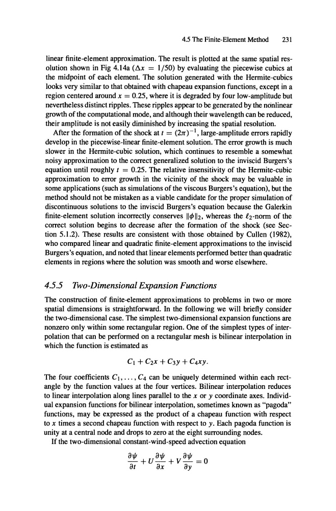
nonzero only within some reetangular region . One of the simplest types of interpolation that can be performed on a reetangular mesh is bilinear interpolation in
which the function is estimated as
The four coefficients CI , ... , C4 can be uniquely determined within each rectangle by the function values at the four vertices . Bilinear interpolation reduces
to linear interpolation along lines parallel to the x or y coordinate axes. Individual expansion functions for bilinear interpolation, sometimes known as "pagoda"
functions , may be expressed as the product of a chapeau function with respect
to x times a second chapeau function with respect to y. Each pagoda function is
unity at a central node and drops to zero at the eight surrounding nodes.
If the two-dimensional constant-wind-speed advection equation
231
linear finite-element approximation. The result is plotted at the same spatial resolution shown in Fig 4.l4a (ßx = I/50) by evaluating the piecewise cubics at
the midpoint of each element. The solution generated with the Hermite-cub ics
looks very similar to that obtained with chapeau expansion functions, except in a
region centered around x = 0.25, where it is degraded by four low-amplitude but
nevertheless distinct ripples. These ripples appear to be generated by the nonlinear
growth of the computational mode, and although their wavelength can be reduced,
their amplitude is not easily diminished by increasing the spatial resolution .
After the formation of the shock at t = (2n) -I, large-amplitude errors rapidly
develop in the piecewise-linear finite-element solution. The error growth is much
slower in the Hermite-cubic solution, which continues to resemble a somewhat
noisy approximation to the correct generalized solution to the inviscid Burgers's
equation until roughly t = 0.25. The relative insensitivity of the Hermite-cubic
approximation to error growth in the vicinity of the shock may be valuable in
some applications (such as simulations ofthe viscous Burgers's equation), but the
method should not be mistaken as a viable candidate for the proper simulation of
discontinuous solutions to the inviscid Burgers's equation because the Galerkin
finite-element solution incorrectly conserves IIcP1I2, whereas the 12-norm of the
correct solution begins to decrease after the formation of the shock (see Section 5.1.2). These results are consistent with those obtained by Cullen (1982),
who compared linear and quadratic finite-element approximations to the inviscid
Burgers 's equation, and noted that linear elements performed better than quadratic
elements in regions where the solution was smooth and worse elsewhere .
4.5.5 Two-Dimensional Expansion Functions
The construction of finite-element approximations to problems in two or more
spatial dimensions is straightforward. In the following we will briefty consider
the two-dimensional case. The simplest two-dimensional expansion functions are
nonzero only within some reetangular region . One of the simplest types of interpolation that can be performed on a reetangular mesh is bilinear interpolation in
which the function is estimated as
The four coefficients CI , ... , C4 can be uniquely determined within each rectangle by the function values at the four vertices . Bilinear interpolation reduces
to linear interpolation along lines parallel to the x or y coordinate axes. Individual expansion functions for bilinear interpolation, sometimes known as "pagoda"
functions , may be expressed as the product of a chapeau function with respect
to x times a second chapeau function with respect to y. Each pagoda function is
unity at a central node and drops to zero at the eight surrounding nodes.
If the two-dimensional constant-wind-speed advection equation