

(b)
230
(a)
4. Series-Expansion Methods
o
x
1 0
x
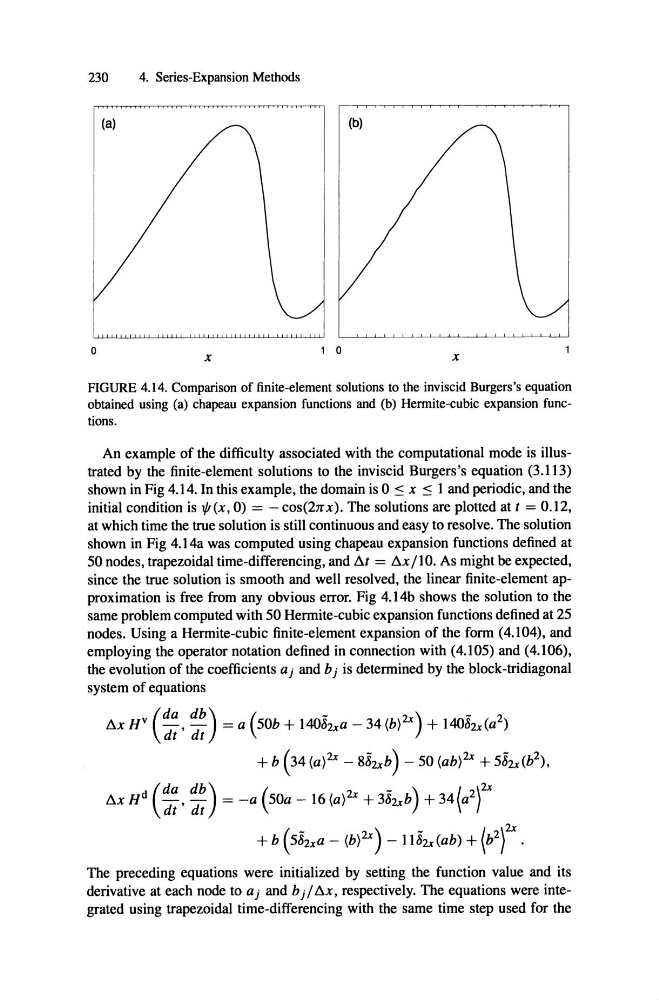
FIGURE 4.14. Comparison of finite-element solutions to the inviscid Burgers's equation
obtained using (a) chapeau expansion functions and (b) Hermite-cubic expansion functions.
An example of the difficulty associated with the computational mode is illustrated by the finite-element solutions to the inviscid Burgers's equation (3.113)
shown in Fig 4.14. In this example, the domain is 0 :5 x :5 1 and periodic, and the
initial condition is 1/1 (x, 0) = - cos(2iT x). The solutions are plotted at I = 0.12,
at which time the true solution is still continuous and easy to resolve. The solution
shown in Fig 4.14a was computed using chapeau expansion functions defined at
SO nodes, trapezoidal time-differencing, and Ar = !i.x/l0. As might be expected,
since the true solution is smooth and weIl resolved, the linear finite-element approximation is free from any obvious error. Fig 4.14b shows the solution to the
same problem computed with SOHerrnite-cubic expansion functions defined at 2S
nodes. Using a Hermite -cubic finite-element expansion of the form (4.104), and
employing the operator notation defined in connection with (4.1OS) and (4.106),
the evolution of the coefficients a j and bj is determined by the block-tridiagonal
system of equations
!i.x H
V
= a (SOb + 14082xa - 34 (b)2x) + 14082xCa2)
+ b (34 (a)2x - 882X b) - SO (ab)2x + S82x(b 2),
= -a (SOa - 16 (a)2x + 382xb) + 34(a2t
+ b (S82Xa - (b)2x) - 1182x(ab) + ( b2 t .
!i.x H
d
The preceding equations were initialized by setting the function value and its
derivative at each node to aj and bj / !i.x , respectively. The equations were integrated using trapezoidal time-differencing with the same time step used for the
230
(a)
4. Series-Expansion Methods
o
x
1 0
x
FIGURE 4.14. Comparison of finite-element solutions to the inviscid Burgers's equation
obtained using (a) chapeau expansion functions and (b) Hermite-cubic expansion functions.
An example of the difficulty associated with the computational mode is illustrated by the finite-element solutions to the inviscid Burgers's equation (3.113)
shown in Fig 4.14. In this example, the domain is 0 :5 x :5 1 and periodic, and the
initial condition is 1/1 (x, 0) = - cos(2iT x). The solutions are plotted at I = 0.12,
at which time the true solution is still continuous and easy to resolve. The solution
shown in Fig 4.14a was computed using chapeau expansion functions defined at
SO nodes, trapezoidal time-differencing, and Ar = !i.x/l0. As might be expected,
since the true solution is smooth and weIl resolved, the linear finite-element approximation is free from any obvious error. Fig 4.14b shows the solution to the
same problem computed with SOHerrnite-cubic expansion functions defined at 2S
nodes. Using a Hermite -cubic finite-element expansion of the form (4.104), and
employing the operator notation defined in connection with (4.1OS) and (4.106),
the evolution of the coefficients a j and bj is determined by the block-tridiagonal
system of equations
!i.x H
V
= a (SOb + 14082xa - 34 (b)2x) + 14082xCa2)
+ b (34 (a)2x - 882X b) - SO (ab)2x + S82x(b 2),
= -a (SOa - 16 (a)2x + 382xb) + 34(a2t
+ b (S82Xa - (b)2x) - 1182x(ab) + ( b2 t .
!i.x H
d
The preceding equations were initialized by setting the function value and its
derivative at each node to aj and bj / !i.x , respectively. The equations were integrated using trapezoidal time-differencing with the same time step used for the