

226
4. Series-Expansion Methods
4.5.4 Hermite-Cubic Expansion Functions
The use of quadratic finite-elements leads to a system of ordinary differential
equations for the function values at each node that are unlike those generated by
typical finite-difference schemes. The contrast between the finite-element method
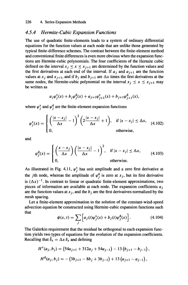
and conventional finite differences is even more obvious when the expansion functions are Hermite-cubic polynomials. The four coefficients of the Hermite cubic
defined on the interval x j
x
x j+ 1 are determined by the function values and
the first derivatives at each end of the interval. If aj and aj+1 are the function
values at x j and x j+I, and if bj and bj+ 1 are t1x times the first derivatives at the
same nodes, the Hermite-cubic polynomial on the interval x j
x
X j+1 may
be written as
where rpj and rp1 are the finite-element expansion functions
I ( Ix - xjl - 1)2 (2 1 X - xjl + 1) if Ix - xjl Sx,
rpj(x) =
Sx
t 1 x '
otherwise,
and
0,
I( X -Xj) (IX -Xjl _1)2,
d
rp/x) =
t1x
Sx
0,
otherwise.
(4.102)
(4.103)
(4.104)
ljJ(X, t) = L [aj(t)rpj(x) +bAt)rp1(x)].
j
As illustrated in Fig . 4.11, rpj has unit amplitude and a zero first derivative at
the jth node , whereas the amplitude of rp1 is zero at x i- but its first derivative
is (t1x)-I . In contrast to linear or quadratic finite-elernent approximations, two
pieces of information are available at each node. The expansion coefficients a j
are the function values at xt- and the bj are the first derivatives normalized by the
mesh spacing.
Let a finite-element approximation to the solution of the constant-wind-speed
advection equation be constructed using Hermite-cubic expansion functions such
that
The Galerkin requirement that the residual be orthogonal to each expansion function yields two types of equations for the evolution of the expansion coefficients.
Recalling that 8 x = t1x Ox and defining
HV(aj, bj) = (54aj+1 + 312aj + 54aj_l) - 13 (bj+1 - bj_I),
Hd(aj , bj) = - (3bj+1 - 8bj + 3bj_l) + 13 (aj+1 - aj_I) ,
4. Series-Expansion Methods
4.5.4 Hermite-Cubic Expansion Functions
The use of quadratic finite-elements leads to a system of ordinary differential
equations for the function values at each node that are unlike those generated by
typical finite-difference schemes. The contrast between the finite-element method
and conventional finite differences is even more obvious when the expansion functions are Hermite-cubic polynomials. The four coefficients of the Hermite cubic
defined on the interval x j
x
x j+ 1 are determined by the function values and
the first derivatives at each end of the interval. If aj and aj+1 are the function
values at x j and x j+I, and if bj and bj+ 1 are t1x times the first derivatives at the
same nodes, the Hermite-cubic polynomial on the interval x j
x
X j+1 may
be written as
where rpj and rp1 are the finite-element expansion functions
I ( Ix - xjl - 1)2 (2 1 X - xjl + 1) if Ix - xjl Sx,
rpj(x) =
Sx
t 1 x '
otherwise,
and
0,
I( X -Xj) (IX -Xjl _1)2,
d
rp/x) =
t1x
Sx
0,
otherwise.
(4.102)
(4.103)
(4.104)
ljJ(X, t) = L [aj(t)rpj(x) +bAt)rp1(x)].
j
As illustrated in Fig . 4.11, rpj has unit amplitude and a zero first derivative at
the jth node , whereas the amplitude of rp1 is zero at x i- but its first derivative
is (t1x)-I . In contrast to linear or quadratic finite-elernent approximations, two
pieces of information are available at each node. The expansion coefficients a j
are the function values at xt- and the bj are the first derivatives normalized by the
mesh spacing.
Let a finite-element approximation to the solution of the constant-wind-speed
advection equation be constructed using Hermite-cubic expansion functions such
that
The Galerkin requirement that the residual be orthogonal to each expansion function yields two types of equations for the evolution of the expansion coefficients.
Recalling that 8 x = t1x Ox and defining
HV(aj, bj) = (54aj+1 + 312aj + 54aj_l) - 13 (bj+1 - bj_I),
Hd(aj , bj) = - (3bj+1 - 8bj + 3bj_l) + 13 (aj+1 - aj_I) ,