

4.5 The Finite-Element Method
WAV ELENGTH
, , , ,
3A
\
:tfU
WAV E NUMBER
5IM
\
\
-------- --- - -- -- ;:.,:,
---. .... "- "- "- " " " , ,
7f1A
.
c*
C
1.0
0.9
0.8
0.7
0.6
0.5
0
\
,
\
\
F1
4E
\
\
\
\
\
\
\
\
\
\
\
\
\
\
\
\
\
225
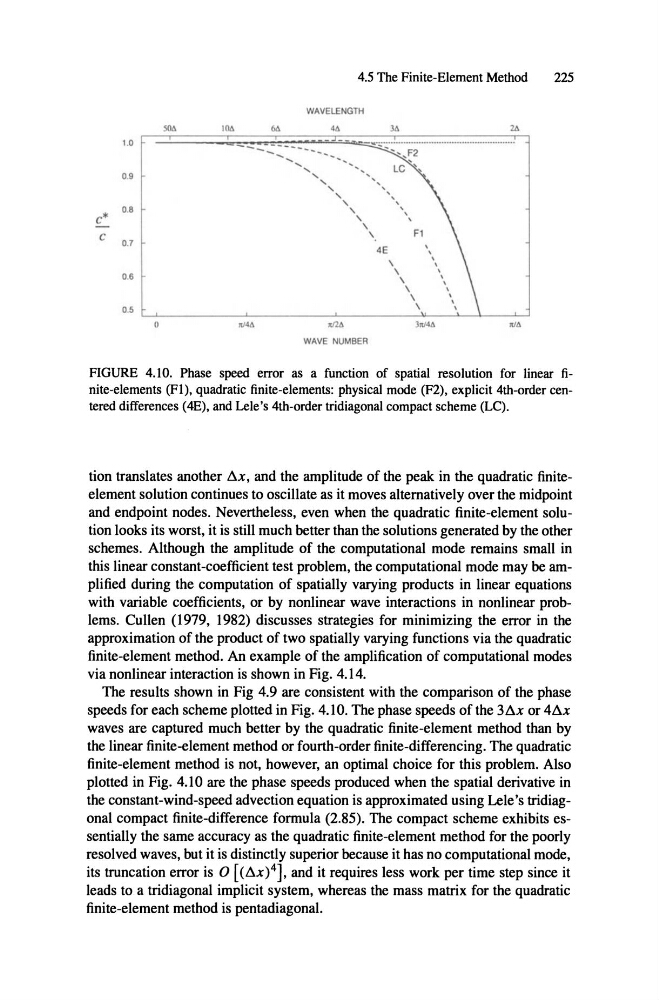
FIGURE 4.10. Phase speed error as a function of spatial resolution for linear finite-elernents (F!), quadratic finite-elements: physical mode (F2), explicit 4th-order centered differences (4E), and Lele's 4th-order tridiagonal compact scheme (LC).
tion translates another !lx, and the amplitude of the peak. in the quadratic finiteelement solution continues to oscillate as it moves altematively over the midpoint
and endpoint nodes . Nevertheless, even when the quadratic finite-element solution looks its worst, it is still much better than the solutions generated by the other
schemes. Although the amplitude of the computational mode remains small in
this linear constant-coefficient test problem, the computational mode may be amplified during the computation of spatially varying products in linear equations
with variable coefficients , or by nonlinear wave interactions in nonlinear problems. Cullen (1979, 1982) discusses strategies for minimizing the error in the
approximation of the product of two spatially varying functions via the quadratic
finite-element method . An example of the amplification of computational modes
via nonlinear interaction is shown in Fig. 4.14.
The results shown in Fig 4.9 are consistent with the comparison of the phase
speeds for each scheme plotted in Fig. 4.10. The phase speeds of the 3!lx or 4!lx
waves are captured much better by the quadratic finite-element method than by
the linear finite-element method or fourth -order finite-differencing. The quadratic
finite-elernent method is not, however, an optimal choice for this problem . Also
plotted in Fig. 4.10 are the phase speeds produced when the spatial derivative in
the constant-wind-speed advection equation is approximated using Lele's tridiagonal compact finite-difference formula (2.85). The compact scheme exhibits essentially the same accuracy as the quadratic finite-element method for the poorly
resolved waves, but it is distinctly superior because it has no computational mode,
its truncation error is 0 [(!lx)4], and it requires less work per time step since it
leads to a tridiagonal implicit system, whereas the mass matrix for the quadratic
finite-elernent method is pentadiagonal.
WAV ELENGTH
, , , ,
3A
\
:tfU
WAV E NUMBER
5IM
\
\
-------- --- - -- -- ;:.,:,
---. .... "- "- "- " " " , ,
7f1A
.
c*
C
1.0
0.9
0.8
0.7
0.6
0.5
0
\
,
\
\
F1
4E
\
\
\
\
\
\
\
\
\
\
\
\
\
\
\
\
\
225
FIGURE 4.10. Phase speed error as a function of spatial resolution for linear finite-elernents (F!), quadratic finite-elements: physical mode (F2), explicit 4th-order centered differences (4E), and Lele's 4th-order tridiagonal compact scheme (LC).
tion translates another !lx, and the amplitude of the peak. in the quadratic finiteelement solution continues to oscillate as it moves altematively over the midpoint
and endpoint nodes . Nevertheless, even when the quadratic finite-element solution looks its worst, it is still much better than the solutions generated by the other
schemes. Although the amplitude of the computational mode remains small in
this linear constant-coefficient test problem, the computational mode may be amplified during the computation of spatially varying products in linear equations
with variable coefficients , or by nonlinear wave interactions in nonlinear problems. Cullen (1979, 1982) discusses strategies for minimizing the error in the
approximation of the product of two spatially varying functions via the quadratic
finite-element method . An example of the amplification of computational modes
via nonlinear interaction is shown in Fig. 4.14.
The results shown in Fig 4.9 are consistent with the comparison of the phase
speeds for each scheme plotted in Fig. 4.10. The phase speeds of the 3!lx or 4!lx
waves are captured much better by the quadratic finite-element method than by
the linear finite-element method or fourth -order finite-differencing. The quadratic
finite-elernent method is not, however, an optimal choice for this problem . Also
plotted in Fig. 4.10 are the phase speeds produced when the spatial derivative in
the constant-wind-speed advection equation is approximated using Lele's tridiagonal compact finite-difference formula (2.85). The compact scheme exhibits essentially the same accuracy as the quadratic finite-element method for the poorly
resolved waves, but it is distinctly superior because it has no computational mode,
its truncation error is 0 [(!lx)4], and it requires less work per time step since it
leads to a tridiagonal implicit system, whereas the mass matrix for the quadratic
finite-elernent method is pentadiagonal.