

222
4. Series-Expansion Methods
o [(ßX)n+J] by piecewise polynomials of order n. Thus, ifthe nodal values could
be specified with negligible error, quadratic expansion functions could provide
o [(ßx)3] accuracy between the nodes. Hut since the quadratic finite-element
method only predicts the nodal values to 0 [(ßx)2], the accuracy between the
nodes is also limited to 0 [(ßx)2]. As discussed in detail by Cullen and Morton
(1980), it is necessary to specify how the error will be measured (e.g ., pointwise
errors at the nodes or the square integral of the error over the entire spatial domain) before attempting to determine the truncation error.
The second, and perhaps more important, reason why the preceding comparison
of truncation error can be misleading is that it does not provide reliable information about the errors in the poorly resolved waves, and in many fluid dynamical
applications, the total error can be dominated by the errors in the shortest waves.
The error in quadratic finite -element solutions to the constant-wind-speed advection equation can be evaluated as a function of the spatial resolution by examining the phase-speed and amplitude errors in semi-discrete wave solutions to (4.97)
and (4.98). There is, however, no single wave ofthe form t/lj(t) = ei(kjl:l.x-wt) that
will simultaneously satisfy (4.97) and (4.98) (Hedstrom 1979a; Cullen 1982). If
the initial disturbance consists of a single wave, at subsequent times the approximate numerical solution will split into two traveling disturbanees. Each disturbance resembles an ordinary traveling wave except that the wave amplitude at the
endpoint nodes is different from that at the midpoint nodes. The nodal values in
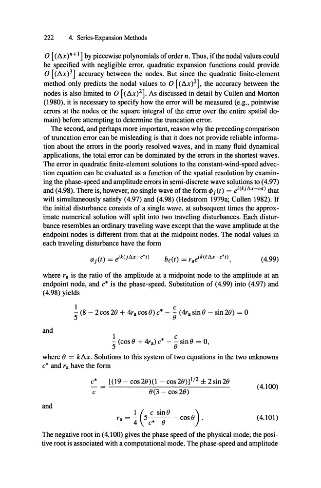
each traveling disturbance have the form
(4.99)
where ra is the ratio of the amplitude at amidpoint node to the amplitude at an
endpoint node, and c* is the phase-speed. Substitution of (4.99) into (4.97) and
(4.98) yields
1
c
.
.
"5 (8 - 2 cos 20 + 4r a cos e) c* - {j (4rasmO - sm20) = 0
and
"5
1 (cos e + 4ra)c * - {j
c smO
. = 0,
where 0 = ktxx , Solutions to this system of two equations in the two unknowns
c* and r a have the form
c*
c
[(19 - cos 20)(1 - cos 20)]1 /2 ± 2 sin20
0(3 - cos20)
(4.100)
and
ra = - I ( 5 -
C - -
sinO - cos 0 ) .
4
c* 0
(4.101)
The negative root in (4.100) gives the phase speed of the physical mode; the positive root is associated with a computational mode. The phase-speed and amplitude
4. Series-Expansion Methods
o [(ßX)n+J] by piecewise polynomials of order n. Thus, ifthe nodal values could
be specified with negligible error, quadratic expansion functions could provide
o [(ßx)3] accuracy between the nodes. Hut since the quadratic finite-element
method only predicts the nodal values to 0 [(ßx)2], the accuracy between the
nodes is also limited to 0 [(ßx)2]. As discussed in detail by Cullen and Morton
(1980), it is necessary to specify how the error will be measured (e.g ., pointwise
errors at the nodes or the square integral of the error over the entire spatial domain) before attempting to determine the truncation error.
The second, and perhaps more important, reason why the preceding comparison
of truncation error can be misleading is that it does not provide reliable information about the errors in the poorly resolved waves, and in many fluid dynamical
applications, the total error can be dominated by the errors in the shortest waves.
The error in quadratic finite -element solutions to the constant-wind-speed advection equation can be evaluated as a function of the spatial resolution by examining the phase-speed and amplitude errors in semi-discrete wave solutions to (4.97)
and (4.98). There is, however, no single wave ofthe form t/lj(t) = ei(kjl:l.x-wt) that
will simultaneously satisfy (4.97) and (4.98) (Hedstrom 1979a; Cullen 1982). If
the initial disturbance consists of a single wave, at subsequent times the approximate numerical solution will split into two traveling disturbanees. Each disturbance resembles an ordinary traveling wave except that the wave amplitude at the
endpoint nodes is different from that at the midpoint nodes. The nodal values in
each traveling disturbance have the form
(4.99)
where ra is the ratio of the amplitude at amidpoint node to the amplitude at an
endpoint node, and c* is the phase-speed. Substitution of (4.99) into (4.97) and
(4.98) yields
1
c
.
.
"5 (8 - 2 cos 20 + 4r a cos e) c* - {j (4rasmO - sm20) = 0
and
"5
1 (cos e + 4ra)c * - {j
c smO
. = 0,
where 0 = ktxx , Solutions to this system of two equations in the two unknowns
c* and r a have the form
c*
c
[(19 - cos 20)(1 - cos 20)]1 /2 ± 2 sin20
0(3 - cos20)
(4.100)
and
ra = - I ( 5 -
C - -
sinO - cos 0 ) .
4
c* 0
(4.101)
The negative root in (4.100) gives the phase speed of the physical mode; the positive root is associated with a computational mode. The phase-speed and amplitude