

WAVELENGTH
M
46
5lM
104
"'6
ll1U
WAVE NUMBER
3"'46
c
"'46
o
c*jc
\
, , , ,
-'-_ _-'-_ _---L..J
, , ,
\
\
\
\
\
\
\
\
\
\
\
3
5
2
O'-'-_ _--'
4.5 The Finite-Element Method
WAVELENGTH
5lM
104
M
46
36
223
...... -1
/ / /
o -- - -
,"
, c'"
..-..- -- .
'------..
o
1II2A
WAVE NUMBER
3"'46
"'6
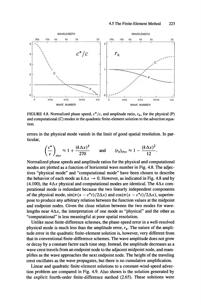
FIGURE 4.8. Nonnalized phase speed, e* je, and amplitude ratio, Ta , for the physical (P)
and computational (C) modes in the quadratic finite-element solution to the advection equation.
errors in the physical mode vanish in the limit of good spatial resolution. In particular,
-
C
phys
270
and
Normalized phase speeds and amplitude ratios for the physical and computational
modes are plotted as a function of horizontal wave number in Fig. 4.8 . The adjectives "physical mode" and "computational mode" have been chosen to describe
the behavior of each mode as k
O. However, as indicated in Fig. 4.8 and by
(4.100), the
physical and computational modes are identical. The
computational mode is redundant because the two linearly independent components
ofthe physical mode, sin(1f(x -
and cos(1f(x -
superimpose to produce any arbitrary relation between the function values at the midpoint
and endpoint nodes. Given the elose relation between the two modes for wavelengths near
the interpretation of one mode as "physical" and the other as
"computational" is less meaningful at poor spatial resolution.
Unlike most finite-difference schemes, the phase-speed error in a well-resolved
physical mode is much less than the amplitude error, Ta. The nature of the amplitude error in the quadratic finite-element solution is, however, very different from
that in conventional finite-difference schemes. The wave amplitude does not grow
or decay by a constant factor each time step. Instead, the amplitude decreases as a
wave crest travels from an endpoint node to the adjacent midpoint node, and reamplifies as the wave approaches the next endpoint node. The height of the traveling
crest oscillates as the wave propagates, but there is no cumulative amplification.
Linear and quadratic finite-element solutions to a constant-wind-speed advection problem are compared in Fig. 4.9. Also shown is the solution generated by
the explicit fourth-order finite-difference method (2.65). These solutions were
M
46
5lM
104
"'6
ll1U
WAVE NUMBER
3"'46
c
"'46
o
c*jc
\
, , , ,
-'-_ _-'-_ _---L..J
, , ,
\
\
\
\
\
\
\
\
\
\
\
3
5
2
O'-'-_ _--'
4.5 The Finite-Element Method
WAVELENGTH
5lM
104
M
46
36
223
...... -1
/ / /
o -- - -
,"
, c'"
..-..- -- .
'------..
o
1II2A
WAVE NUMBER
3"'46
"'6
FIGURE 4.8. Nonnalized phase speed, e* je, and amplitude ratio, Ta , for the physical (P)
and computational (C) modes in the quadratic finite-element solution to the advection equation.
errors in the physical mode vanish in the limit of good spatial resolution. In particular,
-
C
phys
270
and
Normalized phase speeds and amplitude ratios for the physical and computational
modes are plotted as a function of horizontal wave number in Fig. 4.8 . The adjectives "physical mode" and "computational mode" have been chosen to describe
the behavior of each mode as k
O. However, as indicated in Fig. 4.8 and by
(4.100), the
physical and computational modes are identical. The
computational mode is redundant because the two linearly independent components
ofthe physical mode, sin(1f(x -
and cos(1f(x -
superimpose to produce any arbitrary relation between the function values at the midpoint
and endpoint nodes. Given the elose relation between the two modes for wavelengths near
the interpretation of one mode as "physical" and the other as
"computational" is less meaningful at poor spatial resolution.
Unlike most finite-difference schemes, the phase-speed error in a well-resolved
physical mode is much less than the amplitude error, Ta. The nature of the amplitude error in the quadratic finite-element solution is, however, very different from
that in conventional finite-difference schemes. The wave amplitude does not grow
or decay by a constant factor each time step. Instead, the amplitude decreases as a
wave crest travels from an endpoint node to the adjacent midpoint node, and reamplifies as the wave approaches the next endpoint node. The height of the traveling
crest oscillates as the wave propagates, but there is no cumulative amplification.
Linear and quadratic finite-element solutions to a constant-wind-speed advection problem are compared in Fig. 4.9. Also shown is the solution generated by
the explicit fourth-order finite-difference method (2.65). These solutions were