

4.5 The Finite-Element Method
213
The tendency of finite-element approximations to produce implicit algebraic equations is no disadvantage in steady-state problems since the finite-difference approximations to such problems also generate implicit algebraic equations. Moreover, in most steady-state systems the fundamental physical problem can bestated
in a variational form naturally suited for solution via the finite-element technique
(Strang and Fix 1973). Dur interest lies in the application of the finite-elernent
method to tirne-dependent wave-like flows for which variational forms do not
naturally arise. The most useful variational criteria for the equations goveming
most wave-like flows are simply obtained by minimizing the residual as defined
by (4.3). The possible strategies for minimizing the residual are those discussed
in Section 4.1. The collocation strategy will not be examined here since, at least
for piecewise-linear expansion functions, it leads to methods that are identical
to simple finite differences. More interesting algorithms with better conservation
properties can be achieved using the Galerkin requirement that the error be orthogonal to the residual, or equivalently, by minimizing (11 R(cP)112)2.
As discussed in Section 4.1, enforcement of the Galerkin requirement leads to
the system of ordinary differential equations
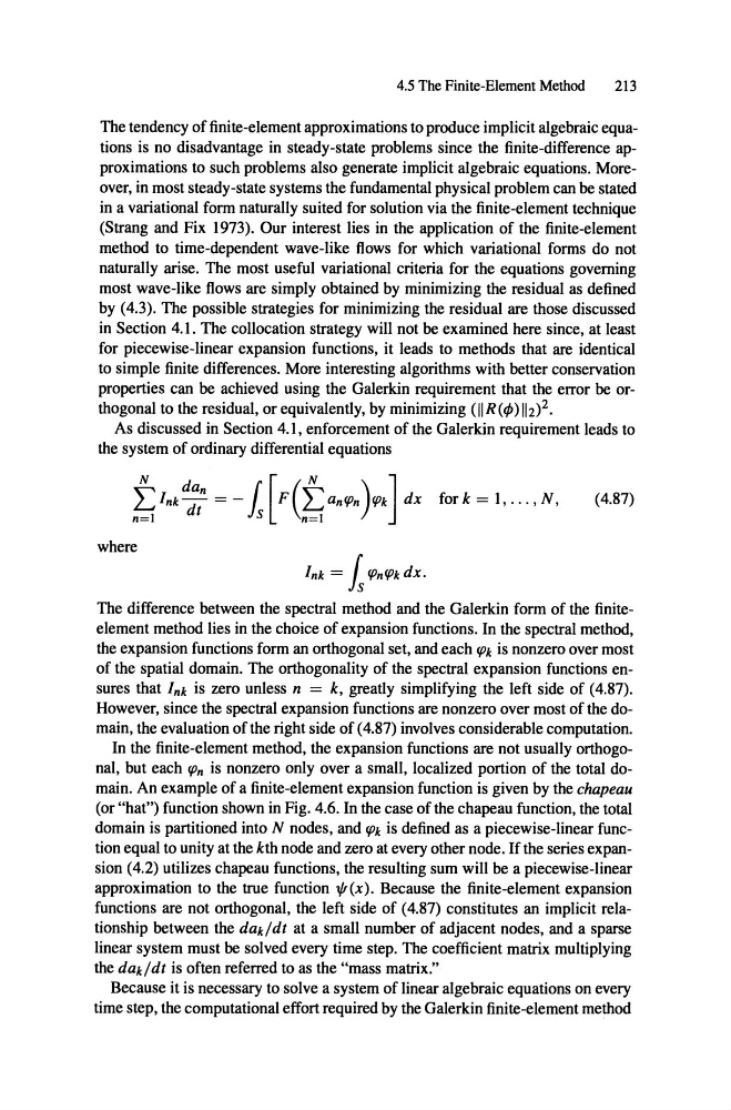
(4.87)
Ink = l rpnrpk dx .
where
The difference between the spectral method and the Galerkin form of the finiteelement method lies in the choice of expansion functions. In the spectral method,
the expansion functions form an orthogonal set, and each rpk is nonzero over most
of the spatial domain. The orthogonality of the spectral expansion functions ensures that Ink is zero unless n = k, greatly simplifying the left side of (4.87).
However, since the spectral expansion functions are nonzero over most of the domain, the evaluation of the right side of (4.87) involves considerable computation.
In the finite-element method, the expansion functions are not usually orthogonal, but each rpn is nonzero only over a smalI, localized portion of the total domain. An example of a finite-element expansion function is given by the chapeau
(or "hat") function shown in Fig. 4.6. In the case of the chapeau function, the total
domain is partitioned into N nodes, and rpk is defined as a piecewise-linear function equal to unity at the kth node and zero at every other node . If the series expansion (4.2) utilizes chapeau functions, the resulting sum will be a piecewise-linear
approximation to the true function 1{I(x). Because the finite-elernent expansion
functions are not orthogonal, the left side of (4.87) constitutes an implicit relationship between the daifdt at a small number of adjacent nodes, and asparse
linear system must be solved every time step. The coefficient matrix multiplying
the daifdt is often referred to as the "mass matrix."
Because it is necessary to solve a system of linear algebraic equations on every
time step, the computational effort required by the Galerkin finite-element method
213
The tendency of finite-element approximations to produce implicit algebraic equations is no disadvantage in steady-state problems since the finite-difference approximations to such problems also generate implicit algebraic equations. Moreover, in most steady-state systems the fundamental physical problem can bestated
in a variational form naturally suited for solution via the finite-element technique
(Strang and Fix 1973). Dur interest lies in the application of the finite-elernent
method to tirne-dependent wave-like flows for which variational forms do not
naturally arise. The most useful variational criteria for the equations goveming
most wave-like flows are simply obtained by minimizing the residual as defined
by (4.3). The possible strategies for minimizing the residual are those discussed
in Section 4.1. The collocation strategy will not be examined here since, at least
for piecewise-linear expansion functions, it leads to methods that are identical
to simple finite differences. More interesting algorithms with better conservation
properties can be achieved using the Galerkin requirement that the error be orthogonal to the residual, or equivalently, by minimizing (11 R(cP)112)2.
As discussed in Section 4.1, enforcement of the Galerkin requirement leads to
the system of ordinary differential equations
(4.87)
Ink = l rpnrpk dx .
where
The difference between the spectral method and the Galerkin form of the finiteelement method lies in the choice of expansion functions. In the spectral method,
the expansion functions form an orthogonal set, and each rpk is nonzero over most
of the spatial domain. The orthogonality of the spectral expansion functions ensures that Ink is zero unless n = k, greatly simplifying the left side of (4.87).
However, since the spectral expansion functions are nonzero over most of the domain, the evaluation of the right side of (4.87) involves considerable computation.
In the finite-element method, the expansion functions are not usually orthogonal, but each rpn is nonzero only over a smalI, localized portion of the total domain. An example of a finite-element expansion function is given by the chapeau
(or "hat") function shown in Fig. 4.6. In the case of the chapeau function, the total
domain is partitioned into N nodes, and rpk is defined as a piecewise-linear function equal to unity at the kth node and zero at every other node . If the series expansion (4.2) utilizes chapeau functions, the resulting sum will be a piecewise-linear
approximation to the true function 1{I(x). Because the finite-elernent expansion
functions are not orthogonal, the left side of (4.87) constitutes an implicit relationship between the daifdt at a small number of adjacent nodes, and asparse
linear system must be solved every time step. The coefficient matrix multiplying
the daifdt is often referred to as the "mass matrix."
Because it is necessary to solve a system of linear algebraic equations on every
time step, the computational effort required by the Galerkin finite-element method