

3.3 Splittinginto FractionalSteps
129
3.3 Splitting into Fractional Steps
More efficient integrat ion schemes can often be obtained by splitting complex
finite-difference formulae into aseries of fractional steps . As an example, the
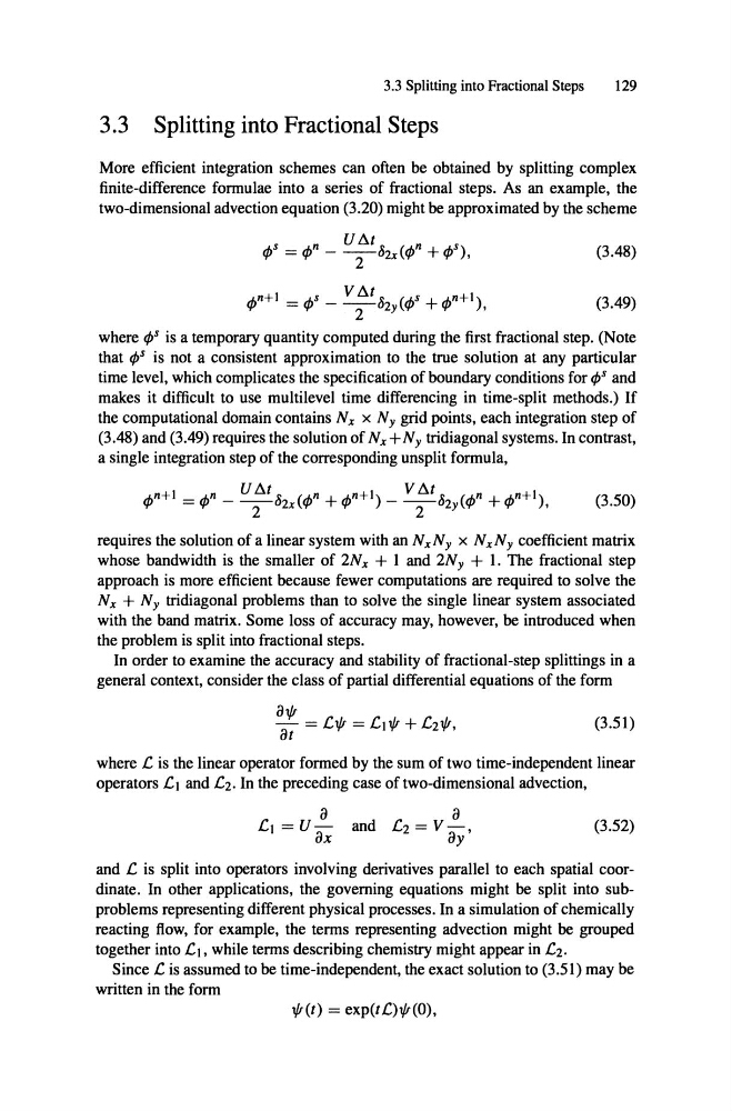
two-dimensional advection equation (3.20) might be approximated by the scheme
r/JS = r/Jn _ U /:::,.t lJzx(r/Jn + r/JS),
r/Jn+1 = r/Js _ V 6.t lJZy(r/Js + r/Jn+l),
2
2
(3.48)
(3.49)
where r/Js is a temporary quantity computed during the first fractional step. (Note
that r/Js is not a consistent approximation to the true solution at any particular
time level, which complicates the specification of boundary conditions for r/Js and
makes it difficult to use multilevel time differencing in time-split methods .) If
the computational domain contains Nx x Ny grid points, each integration step of
(3.48) and (3.49) requires the solution of Nx +Ny tridiagonal systems. In contrast,
a single integration step of the corresponding unsplit formula,
(3.50)
requires the solution of a linear system with an NxNy x NxNy coefficient matrix
whose bandwidth is the smaller of 2N x + 1 and 2N y + 1. The fractional step
approach is more efficient because fewer computations are required to solve the
Nx + Ny tridiagonal problems than to solve the single linear system associated
with the band matrix. Some loss of accuracy may, however, be introduced when
the problem is split into fractional steps .
In order to examine the accuracy and stability of fractional-step splittings in a
general context, consider the dass of partial differential equations of the form
(3.51)
where L is the linear operator formed by the sum of two time -independent linear
operators LI and Lz . In the preceding case of two-dimensional advection,
8
LI = U 8x
8
and LZ = V 8y'
(3.52)
and L is split into operators involving derivatives parallel to each spatial coordinate. In other applications, the goveming equations might be split into subproblems representing different physical processes. In a simulation of chemically
reacting flow, for example, the terms representing advection might be grouped
together into LI, while terms describing chemistry might appear in L2.
Since L is assumed to be time-independent, the exact solution to (3.51) may be
written in the form
1/I(t) = exp(tL)1/I(0) ,
129
3.3 Splitting into Fractional Steps
More efficient integrat ion schemes can often be obtained by splitting complex
finite-difference formulae into aseries of fractional steps . As an example, the
two-dimensional advection equation (3.20) might be approximated by the scheme
r/JS = r/Jn _ U /:::,.t lJzx(r/Jn + r/JS),
r/Jn+1 = r/Js _ V 6.t lJZy(r/Js + r/Jn+l),
2
2
(3.48)
(3.49)
where r/Js is a temporary quantity computed during the first fractional step. (Note
that r/Js is not a consistent approximation to the true solution at any particular
time level, which complicates the specification of boundary conditions for r/Js and
makes it difficult to use multilevel time differencing in time-split methods .) If
the computational domain contains Nx x Ny grid points, each integration step of
(3.48) and (3.49) requires the solution of Nx +Ny tridiagonal systems. In contrast,
a single integration step of the corresponding unsplit formula,
(3.50)
requires the solution of a linear system with an NxNy x NxNy coefficient matrix
whose bandwidth is the smaller of 2N x + 1 and 2N y + 1. The fractional step
approach is more efficient because fewer computations are required to solve the
Nx + Ny tridiagonal problems than to solve the single linear system associated
with the band matrix. Some loss of accuracy may, however, be introduced when
the problem is split into fractional steps .
In order to examine the accuracy and stability of fractional-step splittings in a
general context, consider the dass of partial differential equations of the form
(3.51)
where L is the linear operator formed by the sum of two time -independent linear
operators LI and Lz . In the preceding case of two-dimensional advection,
8
LI = U 8x
8
and LZ = V 8y'
(3.52)
and L is split into operators involving derivatives parallel to each spatial coordinate. In other applications, the goveming equations might be split into subproblems representing different physical processes. In a simulation of chemically
reacting flow, for example, the terms representing advection might be grouped
together into LI, while terms describing chemistry might appear in L2.
Since L is assumed to be time-independent, the exact solution to (3.51) may be
written in the form
1/I(t) = exp(tL)1/I(0) ,