

124
3. Beyondthe One-Way Wave Equation
j
y
y
. ' . ' .
:
J
.:::' J
.. j
1
• 1
': 1
.'
'.
x
o
,
: (d)
0
x
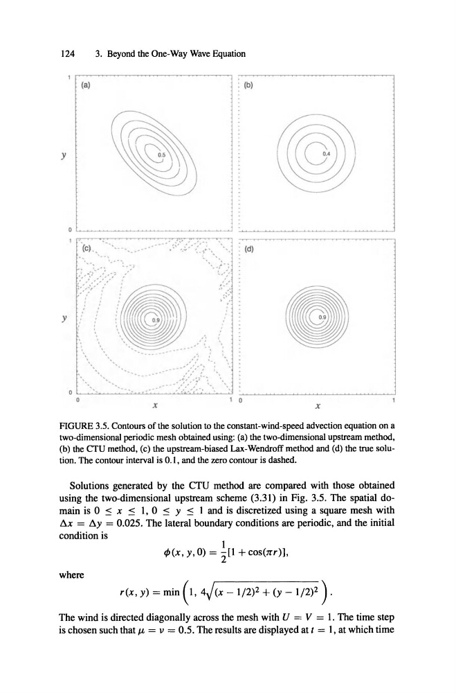
ROURE 3.5. Contours of the solution to the eonstant-wind-speed adveetionequation on a
two-dimensional periodie mesh obtained using: (a) the two-dimensional upstream method,
(b) the CTU method, (e) the upstrearn-biased Lax-Wendroffmethod and (d) the true solution. The eontour interval is 0.1, and the zero eontour is dashed.
Solutions generated by the CTU method are compared with those obtained
using the two-dimensional upstream scheme (3.31) in Fig . 3.5. The spatial domain is 0
x
I, 0
y
land is discretized using a square mesh with
Ax = Ay = 0.025. The lateral boundary conditions are periodic, and the initial
condition is
t/>(x,y,O) = ' 2Y +
1
cos(1l'r)) ,
where
rex, y) = min (I , 4J(x - 1/2)2 + (y - 1/2)2 ).
The wind is directed diagonally across the mesh with U = V = 1. The time step
is chosen such that JL = v = 0.5. The results are displayed at t = I, at which time
3. Beyondthe One-Way Wave Equation
j
y
y
. ' . ' .
:
J
.:::' J
.. j
1
• 1
': 1
.'
'.
x
o
,
: (d)
0
x
ROURE 3.5. Contours of the solution to the eonstant-wind-speed adveetionequation on a
two-dimensional periodie mesh obtained using: (a) the two-dimensional upstream method,
(b) the CTU method, (e) the upstrearn-biased Lax-Wendroffmethod and (d) the true solution. The eontour interval is 0.1, and the zero eontour is dashed.
Solutions generated by the CTU method are compared with those obtained
using the two-dimensional upstream scheme (3.31) in Fig . 3.5. The spatial domain is 0
x
I, 0
y
land is discretized using a square mesh with
Ax = Ay = 0.025. The lateral boundary conditions are periodic, and the initial
condition is
t/>(x,y,O) = ' 2Y +
1
cos(1l'r)) ,
where
rex, y) = min (I , 4J(x - 1/2)2 + (y - 1/2)2 ).
The wind is directed diagonally across the mesh with U = V = 1. The time step
is chosen such that JL = v = 0.5. The results are displayed at t = I, at which time