

3.1 Systems ofEquat ions
115
36
WAVE LENGTH
106
46
_ _ _
--_ .=.:=.;:.:
_
c
w
w
Cl.
:I:
Cl.
c
oL..-'o
----'n/46
----'nIUi
WAVE NUMBER
E
_
.
-'----'
- ' -
3n/46
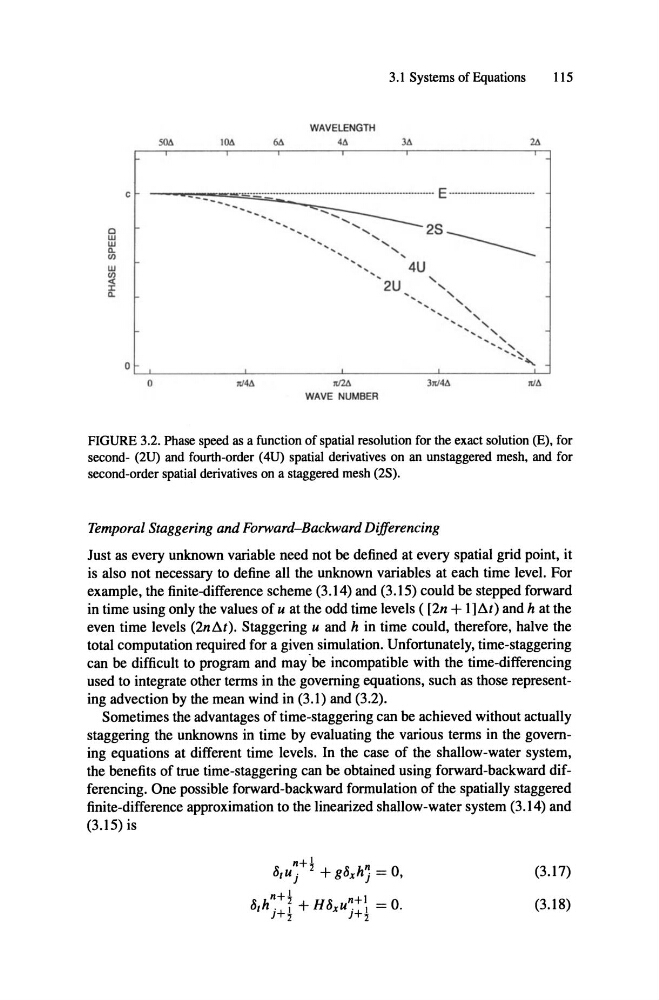
FIGURE 3.2. Phase speed as a function of spatial resolution for the exact solution (E), for
second- (2U) and fourth-order (4U) spatial derivatives on an unstaggered rnesh, and for
second-orderspatial derivatives on a staggered mesh (2S).
Temporal Staggering and Forward-Backward Differencing
Just as every unknown variable need not be defined at every spatial grid point, it
is also not necessary to define all the unknown variables at each time level. For
example, the finite-difference scheme (3.14) and (3.15) could be stepped forward
in time using only the values of u at the odd time levels ( [2n + I]ßt) and hat the
even time levels (2nßt) . Staggering u and h in time could, therefore, halve the
total computation required for a given simulation. Unfortunately, time-staggering
can be difficult to program and may ·be incompatible with the time-differencing
used to integrate other terms in the goveming equations, such as those representing advection by the mean wind in (3.1) and (3.2).
Sometimes the advantages of time-staggering can be achieved without actually
staggering the unknowns in time by evaluating the various terms in the goveming equations at different time levels. In the case of the shallow-water system,
the benefits of true time-staggering can be obtained using forward-backward differencing. One possible forward-backward formulation of the spatially staggered
finite-difference approximation to the linearized shallow-water system (3.14) and
(3.15) is
(3.17)
(3.18)
n
j
n+!
0tU j
+ goxh = 0,
n+!
n+1
Ot h )
"+ 1
1
+ Hoxu "
)+ 1
I = O.
115
36
WAVE LENGTH
106
46
_ _ _
--_ .=.:=.;:.:
_
c
w
w
Cl.
:I:
Cl.
c
oL..-'o
----'n/46
----'nIUi
WAVE NUMBER
E
_
.
-'----'
- ' -
3n/46
FIGURE 3.2. Phase speed as a function of spatial resolution for the exact solution (E), for
second- (2U) and fourth-order (4U) spatial derivatives on an unstaggered rnesh, and for
second-orderspatial derivatives on a staggered mesh (2S).
Temporal Staggering and Forward-Backward Differencing
Just as every unknown variable need not be defined at every spatial grid point, it
is also not necessary to define all the unknown variables at each time level. For
example, the finite-difference scheme (3.14) and (3.15) could be stepped forward
in time using only the values of u at the odd time levels ( [2n + I]ßt) and hat the
even time levels (2nßt) . Staggering u and h in time could, therefore, halve the
total computation required for a given simulation. Unfortunately, time-staggering
can be difficult to program and may ·be incompatible with the time-differencing
used to integrate other terms in the goveming equations, such as those representing advection by the mean wind in (3.1) and (3.2).
Sometimes the advantages of time-staggering can be achieved without actually
staggering the unknowns in time by evaluating the various terms in the goveming equations at different time levels. In the case of the shallow-water system,
the benefits of true time-staggering can be obtained using forward-backward differencing. One possible forward-backward formulation of the spatially staggered
finite-difference approximation to the linearized shallow-water system (3.14) and
(3.15) is
(3.17)
(3.18)
n
j
n+!
0tU j
+ goxh = 0,
n+!
n+1
Ot h )
"+ 1
1
+ Hoxu "
)+ 1
I = O.