

Turbulence and Dispersion of Contaminants in the Planetary Boundary Layer 43
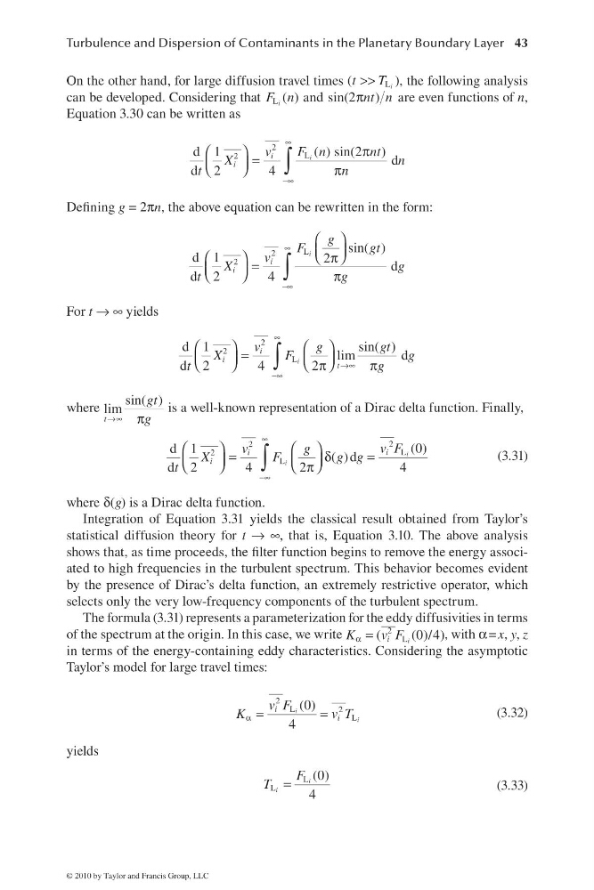
On the other hand, for large diffusion travel times
L
(
)
i
t
T
>>
, the following analysis
can be developed. Considering that L ( )
i
F n and
π
sin(2 )
nt n are even functions of n,
Equation 3.30 can be written as
∞
−∞
π
⎛
⎞ =
⎜
⎟
⎝
⎠
π
∫
2
L
2
( ) sin(2 )
d 1
d
d 2
4
i
i
i
F n
nt
v
X
n
t
n
Defi ning g = 2πn, the above equation can be rewritten in the form:
∞
−∞
⎛ ⎞
⎜ ⎟
⎝ ⎠
⎛
⎞
π
=
⎜
⎟
⎝
⎠
π
∫
L
2
2
sin( )
d 1
2
d
d 2
4
i
i
i
g
F
g t
v
X
g
t
g
For t → ∞ yields
∞
→∞
−∞
⎛
⎞
⎛ ⎞
=
⎜
⎟
⎜ ⎟
⎝
⎠
⎝ ⎠
π
π
∫
2
2
L
d 1
sin( )
lim
d
d 2
4
2
i
i
i
t
v
g
g t
X
F
g
t
g
where
→∞
π
sin( )
lim
t
gt
g
is a well-known representation of a Dirac delta function. Finally,
∞
−∞
⎛
⎞
⎛ ⎞
=
δ
=
⎜
⎟
⎜ ⎟
⎝
⎠
⎝ ⎠
π
∫
2
2
L
2
L
(0)
d 1
( )d
d 2
4
2
4
i
i
i
i
i
v F
v
g
X
F
g g
t
(3.31)
where δ(g) is a Dirac delta function.
Integration of Equation 3.31 yields the classical result obtained from Taylor’s
statistical diffusion theory for t → ∞, that is, Equation 3.10. The above analysis
shows that, as time proceeds, the fi lter function begins to remove the energy associated to high frequencies in the turbulent spectrum. This behavior becomes evident
by the presence of Dirac’s delta function, an extremely restrictive operator, which
selects only the very low-frequency components of the turbulent spectrum.
The formula (3.31) represents a parameterization for the eddy diffusivities in terms
of the spectrum at the origin. In this case, we write
2
L
(
(0)/4)
i
i
K
v F
α =
, with α = x, y, z
in terms of the energy-containing eddy characteristics. Considering the asymptotic
Taylor’s model for large travel times:
α =
=
2
L
2
L
(0)
4
i
i
i
i
v F
K
vT
(3.32)
yields
L
L
(0)
4
i
i
F
T =
(3.33)
© 2010 by Taylor and Francis Group, LLC
On the other hand, for large diffusion travel times
L
(
)
i
t
T
>>
, the following analysis
can be developed. Considering that L ( )
i
F n and
π
sin(2 )
nt n are even functions of n,
Equation 3.30 can be written as
∞
−∞
π
⎛
⎞ =
⎜
⎟
⎝
⎠
π
∫
2
L
2
( ) sin(2 )
d 1
d
d 2
4
i
i
i
F n
nt
v
X
n
t
n
Defi ning g = 2πn, the above equation can be rewritten in the form:
∞
−∞
⎛ ⎞
⎜ ⎟
⎝ ⎠
⎛
⎞
π
=
⎜
⎟
⎝
⎠
π
∫
L
2
2
sin( )
d 1
2
d
d 2
4
i
i
i
g
F
g t
v
X
g
t
g
For t → ∞ yields
∞
→∞
−∞
⎛
⎞
⎛ ⎞
=
⎜
⎟
⎜ ⎟
⎝
⎠
⎝ ⎠
π
π
∫
2
2
L
d 1
sin( )
lim
d
d 2
4
2
i
i
i
t
v
g
g t
X
F
g
t
g
where
→∞
π
sin( )
lim
t
gt
g
is a well-known representation of a Dirac delta function. Finally,
∞
−∞
⎛
⎞
⎛ ⎞
=
δ
=
⎜
⎟
⎜ ⎟
⎝
⎠
⎝ ⎠
π
∫
2
2
L
2
L
(0)
d 1
( )d
d 2
4
2
4
i
i
i
i
i
v F
v
g
X
F
g g
t
(3.31)
where δ(g) is a Dirac delta function.
Integration of Equation 3.31 yields the classical result obtained from Taylor’s
statistical diffusion theory for t → ∞, that is, Equation 3.10. The above analysis
shows that, as time proceeds, the fi lter function begins to remove the energy associated to high frequencies in the turbulent spectrum. This behavior becomes evident
by the presence of Dirac’s delta function, an extremely restrictive operator, which
selects only the very low-frequency components of the turbulent spectrum.
The formula (3.31) represents a parameterization for the eddy diffusivities in terms
of the spectrum at the origin. In this case, we write
2
L
(
(0)/4)
i
i
K
v F
α =
, with α = x, y, z
in terms of the energy-containing eddy characteristics. Considering the asymptotic
Taylor’s model for large travel times:
α =
=
2
L
2
L
(0)
4
i
i
i
i
v F
K
vT
(3.32)
yields
L
L
(0)
4
i
i
F
T =
(3.33)
© 2010 by Taylor and Francis Group, LLC