

Atmospheric Boundary Layer: Concepts and Measurements
25
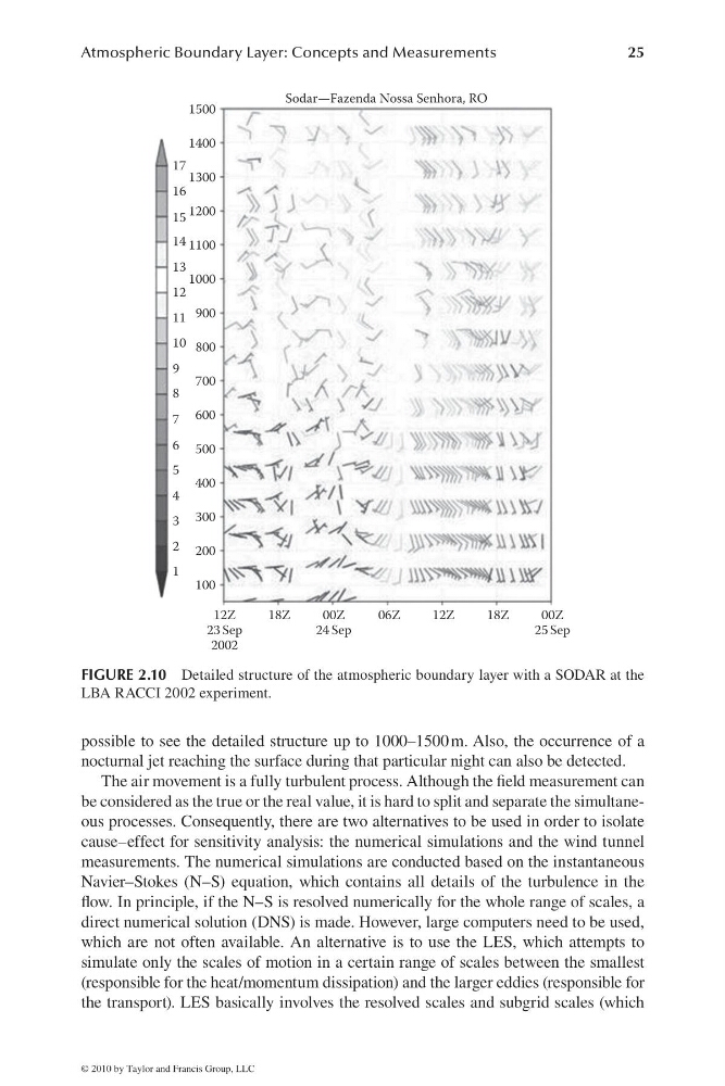
possible to see the detailed structure up to 1000–1500 m. Also, the occurrence of a
nocturnal jet reaching the surface during that particular night can also be detected.
The air movement is a fully turbulent process. Although the fi eld measurement can
be considered as the true or the real value, it is hard to split and separate the simultaneous processes. Consequently, there are two alternatives to be used in order to isolate
cause–effect for sensitivity analysis: the numerical simulations and the wind tunnel
measurements. The numerical simulations are conducted based on the instantaneous
Navier–Stokes (N–S) equation, which contains all details of the turbulence in the
fl ow. In principle, if the N–S is resolved numerically for the whole range of scales, a
direct numerical solution (DNS) is made. However, large computers need to be used,
which are not often available. An alternative is to use the LES, which attempts to
simulate only the scales of motion in a certain range of scales between the smallest
(responsible for the heat/momentum dissipation) and the larger eddies (responsible for
the transport). LES basically involves the resolved scales and subgrid scales (which
1500
1400
1300
1200
1100
1000
900
800
700
600
500
400
300
200
100
12Z
23 Sep
2002
18Z
00Z
24 Sep
06Z
12Z
18Z
00Z
25 Sep
Sodar—Fazenda Nossa Senhora, RO
17
16
15
14
13
12
11
10
9
8
7
6
5
4
3
2
1
FIGURE 2.10 Detailed structure of the atmospheric boundary layer with a SODAR at the
LBA RACCI 2002 experiment.
© 2010 by Taylor and Francis Group, LLC
25
possible to see the detailed structure up to 1000–1500 m. Also, the occurrence of a
nocturnal jet reaching the surface during that particular night can also be detected.
The air movement is a fully turbulent process. Although the fi eld measurement can
be considered as the true or the real value, it is hard to split and separate the simultaneous processes. Consequently, there are two alternatives to be used in order to isolate
cause–effect for sensitivity analysis: the numerical simulations and the wind tunnel
measurements. The numerical simulations are conducted based on the instantaneous
Navier–Stokes (N–S) equation, which contains all details of the turbulence in the
fl ow. In principle, if the N–S is resolved numerically for the whole range of scales, a
direct numerical solution (DNS) is made. However, large computers need to be used,
which are not often available. An alternative is to use the LES, which attempts to
simulate only the scales of motion in a certain range of scales between the smallest
(responsible for the heat/momentum dissipation) and the larger eddies (responsible for
the transport). LES basically involves the resolved scales and subgrid scales (which
1500
1400
1300
1200
1100
1000
900
800
700
600
500
400
300
200
100
12Z
23 Sep
2002
18Z
00Z
24 Sep
06Z
12Z
18Z
00Z
25 Sep
Sodar—Fazenda Nossa Senhora, RO
17
16
15
14
13
12
11
10
9
8
7
6
5
4
3
2
1
FIGURE 2.10 Detailed structure of the atmospheric boundary layer with a SODAR at the
LBA RACCI 2002 experiment.
© 2010 by Taylor and Francis Group, LLC