

20
Air Pollution and Turbulence: Modeling and Applications
a data acquisition system. For the engineering purposes, 10 min averages are recommended, especially for the winds. Within this timescale, the average windspeed, the
mean wind vector (made with the mean horizontal [zonal and meridional] windspeed
components), gust factor, and turbulence intensity can be computed.
For the fl uctuations measurements, the time response of the sensor is the most
important issue to be considered. In order to measure the turbulent fl uxes using the
eddy covariance technique (see Arya, 2001 or Garrat, 1992), a sample rate in the
range 10–20 Hz should be used. Usually, a tridimensional sonic anemometer (with
or without a direct measurement of the air temperature) can be installed at 10 m
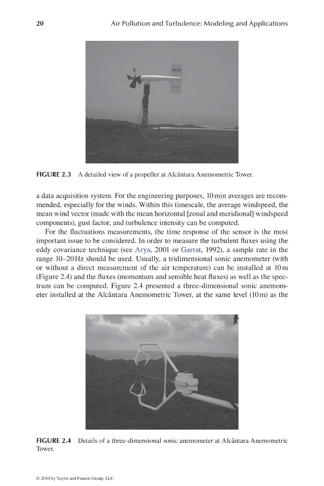
(Figure 2.4) and the fl uxes (momentum and sensible heat fl uxes) as well as the spectrum can be computed. Figure 2.4 presented a three-dimensional sonic anemometer installed at the Alcântara Anemometric Tower, at the same level (10 m) as the
FIGURE 2.3 A detailed view of a propeller at Alcântara Anemometric Tower.
FIGURE 2.4 Details of a three-dimensional sonic anemometer at Alcântara Anemometric
Tower.
© 2010 by Taylor and Francis Group, LLC
Air Pollution and Turbulence: Modeling and Applications
a data acquisition system. For the engineering purposes, 10 min averages are recommended, especially for the winds. Within this timescale, the average windspeed, the
mean wind vector (made with the mean horizontal [zonal and meridional] windspeed
components), gust factor, and turbulence intensity can be computed.
For the fl uctuations measurements, the time response of the sensor is the most
important issue to be considered. In order to measure the turbulent fl uxes using the
eddy covariance technique (see Arya, 2001 or Garrat, 1992), a sample rate in the
range 10–20 Hz should be used. Usually, a tridimensional sonic anemometer (with
or without a direct measurement of the air temperature) can be installed at 10 m
(Figure 2.4) and the fl uxes (momentum and sensible heat fl uxes) as well as the spectrum can be computed. Figure 2.4 presented a three-dimensional sonic anemometer installed at the Alcântara Anemometric Tower, at the same level (10 m) as the
FIGURE 2.3 A detailed view of a propeller at Alcântara Anemometric Tower.
FIGURE 2.4 Details of a three-dimensional sonic anemometer at Alcântara Anemometric
Tower.
© 2010 by Taylor and Francis Group, LLC