

244
Air Pollution and Turbulence: Modeling and Applications
∂
∂
∂ τ
= −
−
+
∂
∂
∂
ci
i
i
i
C
u
S
C
t
x
x
(9.9)
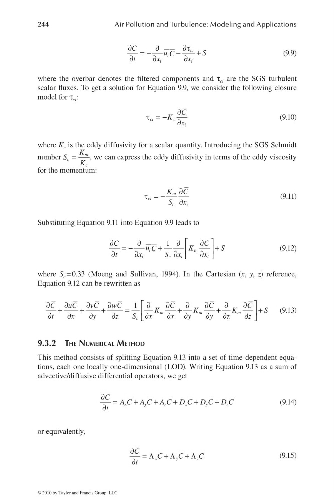
where the overbar denotes the fi ltered components and τ ci are the SGS turbulent
scalar fl uxes. To get a solution for Equation 9.9, we consider the following closure
model for τ ci :
ci
c
i
C
K
x
∂
τ = − ∂
(9.10)
where K c is the eddy diffusivity for a scalar quantity. Introducing the SGS Schmidt
number
m
c
c
K
S
K
=
, we can express the eddy diffusivity in terms of the eddy viscosity
for the momentum:
m
ci
c
i
K C
S x
∂
τ = −
∂
(9.11)
Substituting Equation 9.11 into Equation 9.9 leads to
⎡
⎤
∂
∂
∂
∂
= −
+
+
⎢
⎥
∂
∂
∂
∂
⎣
⎦
1
i
m
i
c
i
i
C
C
u
K
S
C
t
x
S x
x
(9.12)
where S c = 0.33 (Moeng and Sullivan, 1994). In the Cartesian (x, y, z) reference,
Equation 9.12 can be rewritten as
1
m
m
m
c
C
uC
vC
wC
C
C
C
K
K
K
S
t
x
y
z
S
x
x
y
y
z
z
⎡
⎤
∂
∂
∂
∂
∂
∂
∂
∂
∂
∂
+
+
+
=
+
+
+
⎢
⎥
∂
∂
∂
∂
∂
∂
∂
∂
∂
∂
⎣
⎦
(9.13)
9.3.2 THE NUMERICAL METHOD
This method consists of splitting Equation 9.13 into a set of time-dependent equations, each one locally one-dimensional (LOD). Writing Equation 9.13 as a sum of
advective/diffusive differential operators, we get
x
y
z
x
y
z
C A C A C A C D C D C D C
t
∂ =
+
+
+
+
+
∂
(9.14)
or equivalently,
x
y
z
C
C
C
C
t
∂ = Λ + Λ + Λ
∂
(9.15)
© 2010 by Taylor and Francis Group, LLC
Air Pollution and Turbulence: Modeling and Applications
∂
∂
∂ τ
= −
−
+
∂
∂
∂
ci
i
i
i
C
u
S
C
t
x
x
(9.9)
where the overbar denotes the fi ltered components and τ ci are the SGS turbulent
scalar fl uxes. To get a solution for Equation 9.9, we consider the following closure
model for τ ci :
ci
c
i
C
K
x
∂
τ = − ∂
(9.10)
where K c is the eddy diffusivity for a scalar quantity. Introducing the SGS Schmidt
number
m
c
c
K
S
K
=
, we can express the eddy diffusivity in terms of the eddy viscosity
for the momentum:
m
ci
c
i
K C
S x
∂
τ = −
∂
(9.11)
Substituting Equation 9.11 into Equation 9.9 leads to
⎡
⎤
∂
∂
∂
∂
= −
+
+
⎢
⎥
∂
∂
∂
∂
⎣
⎦
1
i
m
i
c
i
i
C
C
u
K
S
C
t
x
S x
x
(9.12)
where S c = 0.33 (Moeng and Sullivan, 1994). In the Cartesian (x, y, z) reference,
Equation 9.12 can be rewritten as
1
m
m
m
c
C
uC
vC
wC
C
C
C
K
K
K
S
t
x
y
z
S
x
x
y
y
z
z
⎡
⎤
∂
∂
∂
∂
∂
∂
∂
∂
∂
∂
+
+
+
=
+
+
+
⎢
⎥
∂
∂
∂
∂
∂
∂
∂
∂
∂
∂
⎣
⎦
(9.13)
9.3.2 THE NUMERICAL METHOD
This method consists of splitting Equation 9.13 into a set of time-dependent equations, each one locally one-dimensional (LOD). Writing Equation 9.13 as a sum of
advective/diffusive differential operators, we get
x
y
z
x
y
z
C A C A C A C D C D C D C
t
∂ =
+
+
+
+
+
∂
(9.14)
or equivalently,
x
y
z
C
C
C
C
t
∂ = Λ + Λ + Λ
∂
(9.15)
© 2010 by Taylor and Francis Group, LLC