

Atmospheric Dispersion with a Large-Eddy Simulation
243
where
2
2
S
U
u v
=
+
u * is the friction velocity
φ m is the Monin–Obukhov stability function for the moment
z = z 1 is the height of the fi rst grid point
κ is the von Karman constant
The SGS vertical fl uxes at the surface are also assigned.
9.2.5 UPPER BOUNDARY CONDITIONS
The top boundary conditions are zero vertical velocity (
–
w = 0), zero SGS turbulence
fi elds, and
0
u
z
∂ =
∂
0
v
z
∂ =
∂
const
z
∂θ =
∂
across the
–
w = 0 level. These kinds of conditions do not allow the transmission of
gravity waves, which can be generated in the stably stratifi ed layer due to turbulent
motions in the PBL. Besides, the upper boundary of a typical LES domain is set to be
well above the PBL top where artifi cial upper boundary conditions on the simulated
PBL may arise.
9.3 EULERIAN DISPERSION WITH LARGE-EDDY
SIMULATIONS AND EXPERIMENTS
9.3.1 EULERIAN DISPERSION
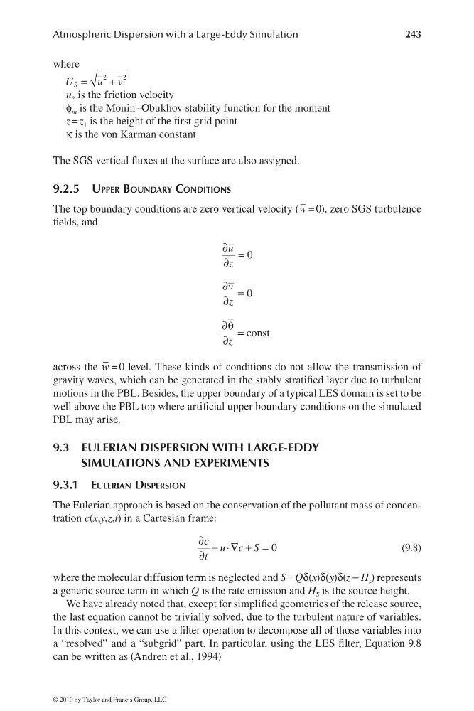
The Eulerian approach is based on the conservation of the pollutant mass of concentration c(x,y,z,t) in a Cartesian frame:
0
c u c S
t
∂ + ⋅∇ + =
∂
(9.8)
where the molecular diffusion term is neglected and S = Qδ(x)δ(y)δ(z − H s ) represents
a generic source term in which Q is the rate emission and H S is the source height.
We have already noted that, except for simplifi ed geometries of the release source,
the last equation cannot be trivially solved, due to the turbulent nature of variables.
In this context, we can use a fi lter operation to decompose all of those variables into
a “resolved” and a “subgrid” part. In particular, using the LES fi lter, Equation 9.8
can be written as (Andren et al., 1994)
© 2010 by Taylor and Francis Group, LLC
243
where
2
2
S
U
u v
=
+
u * is the friction velocity
φ m is the Monin–Obukhov stability function for the moment
z = z 1 is the height of the fi rst grid point
κ is the von Karman constant
The SGS vertical fl uxes at the surface are also assigned.
9.2.5 UPPER BOUNDARY CONDITIONS
The top boundary conditions are zero vertical velocity (
–
w = 0), zero SGS turbulence
fi elds, and
0
u
z
∂ =
∂
0
v
z
∂ =
∂
const
z
∂θ =
∂
across the
–
w = 0 level. These kinds of conditions do not allow the transmission of
gravity waves, which can be generated in the stably stratifi ed layer due to turbulent
motions in the PBL. Besides, the upper boundary of a typical LES domain is set to be
well above the PBL top where artifi cial upper boundary conditions on the simulated
PBL may arise.
9.3 EULERIAN DISPERSION WITH LARGE-EDDY
SIMULATIONS AND EXPERIMENTS
9.3.1 EULERIAN DISPERSION
The Eulerian approach is based on the conservation of the pollutant mass of concentration c(x,y,z,t) in a Cartesian frame:
0
c u c S
t
∂ + ⋅∇ + =
∂
(9.8)
where the molecular diffusion term is neglected and S = Qδ(x)δ(y)δ(z − H s ) represents
a generic source term in which Q is the rate emission and H S is the source height.
We have already noted that, except for simplifi ed geometries of the release source,
the last equation cannot be trivially solved, due to the turbulent nature of variables.
In this context, we can use a fi lter operation to decompose all of those variables into
a “resolved” and a “subgrid” part. In particular, using the LES fi lter, Equation 9.8
can be written as (Andren et al., 1994)
© 2010 by Taylor and Francis Group, LLC