

242
Air Pollution and Turbulence: Modeling and Applications
of view of homogeneity, atmospheric turbulence may have completely different
behaviors in the horizontal and vertical directions. The near-homogeneity in any
horizontal plane allows the application of periodic boundary conditions in both the
x- and the y-directions. On the other hand, in the vertical direction, sources and sinks
of turbulence are not uniformly distributed. A mixed scheme of Fourier expansion in
the horizontal plane and fi nite differencing in the vertical is then appropriate for the
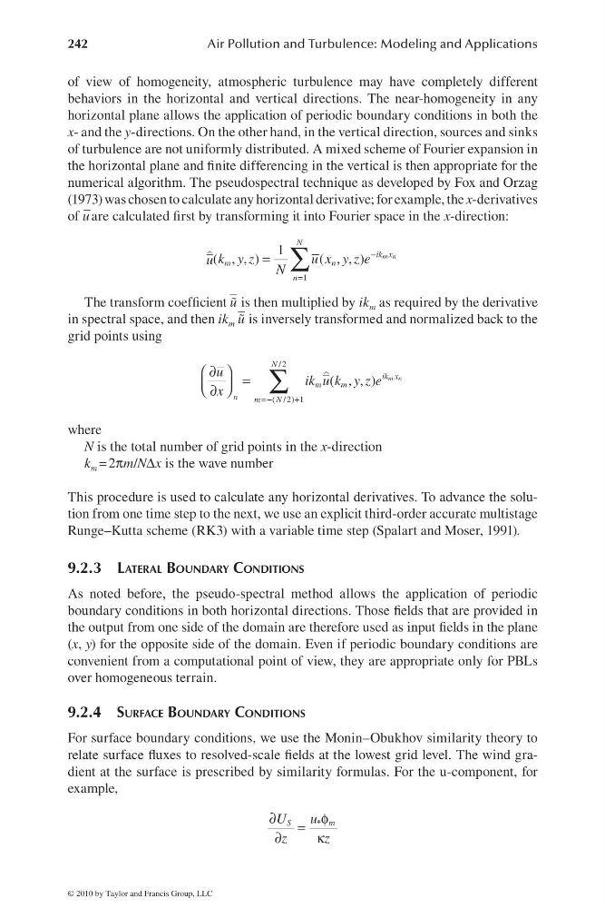
numerical algorithm. The pseudospectral technique as developed by Fox and Orzag
(1973) was chosen to calculate any horizontal derivative; for example, the x-derivatives
of u
– are calculated fi rst by transforming it into Fourier space in the x-direction:
−
=
= ∑
1
1
( , , )
( , , )
m n
N
ik x
m
n
n
k y z
u x y z e
u
N
The transform coeffi cient
–
˜
u is then multiplied by ik m as required by the derivative
in spectral space, and then ik m
–
˜
u is inversely transformed and normalized back to the
grid points using
/2
( /2) 1
( , , )
m n
N
ik x
m
m
n
m
N
u
ik u k y z e
x
=−
+
∂
⎛ ⎞ =
⎜ ⎟
⎝ ⎠
∂
∑
where
N is the total number of grid points in the x-direction
k m = 2πm/NΔx is the wave number
This procedure is used to calculate any horizontal derivatives. To advance the solution from one time step to the next, we use an explicit third-order accurate multistage
Runge–Kutta scheme (RK3) with a variable time step (Spalart and Moser, 1991).
9.2.3 LATERAL BOUNDARY CONDITIONS
As noted before, the pseudo-spectral method allows the application of periodic
boundary conditions in both horizontal directions. Those fi elds that are provided in
the output from one side of the domain are therefore used as input fi elds in the plane
(x, y) for the opposite side of the domain. Even if periodic boundary conditions are
convenient from a computational point of view, they are appropriate only for PBLs
over homogeneous terrain.
9.2.4 SURFACE BOUNDARY CONDITIONS
For surface boundary conditions, we use the Monin–Obukhov similarity theory to
relate surface fl uxes to resolved-scale fi elds at the lowest grid level. The wind gradient at the surface is prescribed by similarity formulas. For the u-component, for
example,
*
S
m
U
u
z
z
∂
φ
=
∂
κ
© 2010 by Taylor and Francis Group, LLC
Air Pollution and Turbulence: Modeling and Applications
of view of homogeneity, atmospheric turbulence may have completely different
behaviors in the horizontal and vertical directions. The near-homogeneity in any
horizontal plane allows the application of periodic boundary conditions in both the
x- and the y-directions. On the other hand, in the vertical direction, sources and sinks
of turbulence are not uniformly distributed. A mixed scheme of Fourier expansion in
the horizontal plane and fi nite differencing in the vertical is then appropriate for the
numerical algorithm. The pseudospectral technique as developed by Fox and Orzag
(1973) was chosen to calculate any horizontal derivative; for example, the x-derivatives
of u
– are calculated fi rst by transforming it into Fourier space in the x-direction:
−
=
= ∑
1
1
( , , )
( , , )
m n
N
ik x
m
n
n
k y z
u x y z e
u
N
The transform coeffi cient
–
˜
u is then multiplied by ik m as required by the derivative
in spectral space, and then ik m
–
˜
u is inversely transformed and normalized back to the
grid points using
/2
( /2) 1
( , , )
m n
N
ik x
m
m
n
m
N
u
ik u k y z e
x
=−
+
∂
⎛ ⎞ =
⎜ ⎟
⎝ ⎠
∂
∑
where
N is the total number of grid points in the x-direction
k m = 2πm/NΔx is the wave number
This procedure is used to calculate any horizontal derivatives. To advance the solution from one time step to the next, we use an explicit third-order accurate multistage
Runge–Kutta scheme (RK3) with a variable time step (Spalart and Moser, 1991).
9.2.3 LATERAL BOUNDARY CONDITIONS
As noted before, the pseudo-spectral method allows the application of periodic
boundary conditions in both horizontal directions. Those fi elds that are provided in
the output from one side of the domain are therefore used as input fi elds in the plane
(x, y) for the opposite side of the domain. Even if periodic boundary conditions are
convenient from a computational point of view, they are appropriate only for PBLs
over homogeneous terrain.
9.2.4 SURFACE BOUNDARY CONDITIONS
For surface boundary conditions, we use the Monin–Obukhov similarity theory to
relate surface fl uxes to resolved-scale fi elds at the lowest grid level. The wind gradient at the surface is prescribed by similarity formulas. For the u-component, for
example,
*
S
m
U
u
z
z
∂
φ
=
∂
κ
© 2010 by Taylor and Francis Group, LLC