

Atmospheric Dispersion with a Large-Eddy Simulation
245
where
x
x
x
m
y
y
y
m
z
z
z
m
A D
u
K
x
x
x
A D
v
K
y
y
y
A D
w
K
z
z
z
⎧
∂
∂
∂
⎛
⎞
Λ = +
≡ −
+ ⎜
⎟
⎪
⎝
⎠
∂
∂
∂
⎪
⎪
⎛
⎞
∂
∂
∂
⎪ Λ = +
≡ −
+
⎨
⎜
⎟
∂
∂
∂
⎝
⎠
⎪
⎪
∂
∂
∂
⎛
⎞
⎪ Λ = +
≡ −
+ ⎜
⎟
⎪
⎝
⎠
∂
∂
∂
⎩
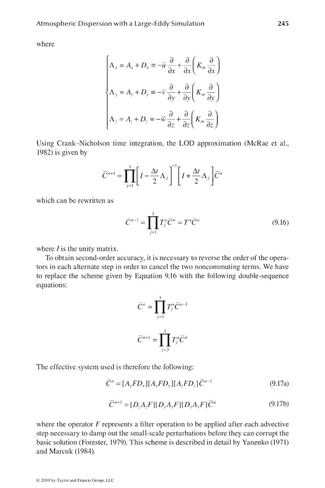
Using Crank–Nicholson time integration, the LOD approximation (McRae et al.,
1982) is given by
1
3
1
1
2
2
n
n
j
j
j
t
t
C
I
I
C
−
+
=
Δ
Δ
⎡
⎤ ⎡
⎤
=
− Λ
+
Λ
⎢
⎥ ⎢
⎥
⎣
⎦ ⎣
⎦
∏
which can be rewritten as
3
1
1
n
n n
n n
j
j
C
TC
TC
+
=
=
=
∏
(9.16)
where I is the unity matrix.
To obtain second-order accuracy, it is necessary to reverse the order of the operators in each alternate step in order to cancel the two noncommuting terms. We have
to replace the scheme given by Equation 9.16 with the following double-sequence
equations:
3
1
1
n
n n
j
j
C
T C
−
=
= ∏
1
1
3
n
n n
j
j
C
TC
+
=
= ∏
The effective system used is therefore the following:
1
[
][
][
]
n
n
x
x
y
y
z
z
C
A FD A FD A FD C
−
=
(9.17a)
1
[
][
][
]
n
n
z z
y y
x x
C
DAF D AF D AF C
+
=
(9.17b)
where the operator F represents a fi lter operation to be applied after each advective
step necessary to damp out the small-scale perturbations before they can corrupt the
basic solution (Forester, 1979). This scheme is described in detail by Yanenko (1971)
and Marcuk (1984).
© 2010 by Taylor and Francis Group, LLC
245
where
x
x
x
m
y
y
y
m
z
z
z
m
A D
u
K
x
x
x
A D
v
K
y
y
y
A D
w
K
z
z
z
⎧
∂
∂
∂
⎛
⎞
Λ = +
≡ −
+ ⎜
⎟
⎪
⎝
⎠
∂
∂
∂
⎪
⎪
⎛
⎞
∂
∂
∂
⎪ Λ = +
≡ −
+
⎨
⎜
⎟
∂
∂
∂
⎝
⎠
⎪
⎪
∂
∂
∂
⎛
⎞
⎪ Λ = +
≡ −
+ ⎜
⎟
⎪
⎝
⎠
∂
∂
∂
⎩
Using Crank–Nicholson time integration, the LOD approximation (McRae et al.,
1982) is given by
1
3
1
1
2
2
n
n
j
j
j
t
t
C
I
I
C
−
+
=
Δ
Δ
⎡
⎤ ⎡
⎤
=
− Λ
+
Λ
⎢
⎥ ⎢
⎥
⎣
⎦ ⎣
⎦
∏
which can be rewritten as
3
1
1
n
n n
n n
j
j
C
TC
TC
+
=
=
=
∏
(9.16)
where I is the unity matrix.
To obtain second-order accuracy, it is necessary to reverse the order of the operators in each alternate step in order to cancel the two noncommuting terms. We have
to replace the scheme given by Equation 9.16 with the following double-sequence
equations:
3
1
1
n
n n
j
j
C
T C
−
=
= ∏
1
1
3
n
n n
j
j
C
TC
+
=
= ∏
The effective system used is therefore the following:
1
[
][
][
]
n
n
x
x
y
y
z
z
C
A FD A FD A FD C
−
=
(9.17a)
1
[
][
][
]
n
n
z z
y y
x x
C
DAF D AF D AF C
+
=
(9.17b)
where the operator F represents a fi lter operation to be applied after each advective
step necessary to damp out the small-scale perturbations before they can corrupt the
basic solution (Forester, 1979). This scheme is described in detail by Yanenko (1971)
and Marcuk (1984).
© 2010 by Taylor and Francis Group, LLC