

220
Air Pollution and Turbulence: Modeling and Applications
This equation, derived by Anfossi (1985), which describes both the transitional
and fi nal phases and different stability conditions, is simply a generalization of the
well-known and validated Briggs’s formulas (1975).
Then, to each ith particle a buoyancy fl ux
i
b
F is assigned at the stack exit, from a
normal distribution having the mean value equal to the mean buoyancy fl ux b
F and
the standard deviation equal to
3
b
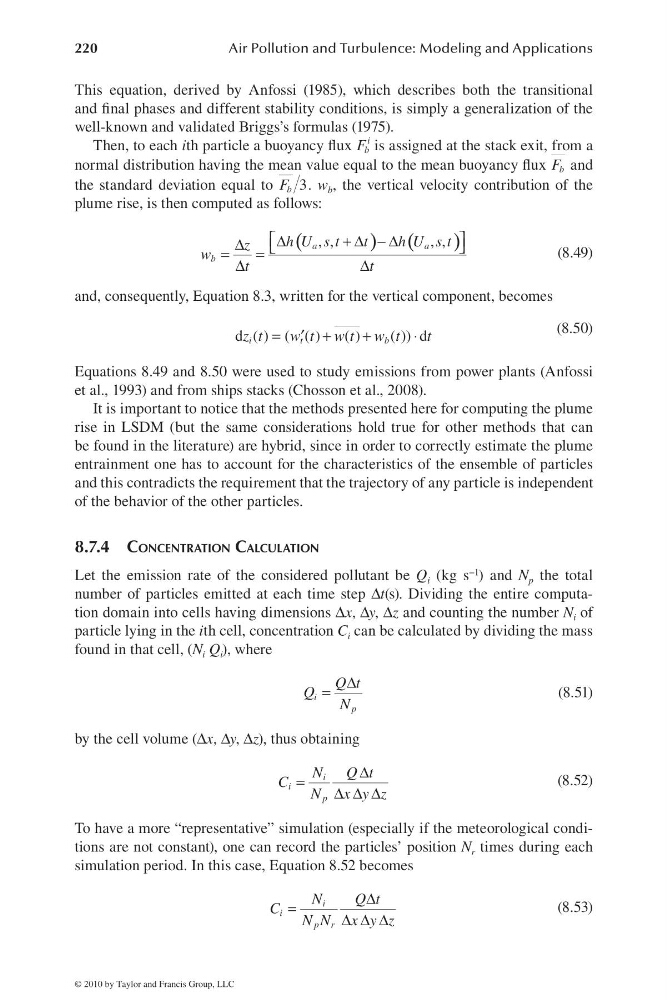
F . w b , the vertical velocity contribution of the
plume rise, is then computed as follows:
(
) (
)
, ,
, ,
a
a
b
h U s t
t
h U s t
z
w
t
t
⎡
⎤
Δ
+Δ −Δ
Δ
⎣
⎦
=
=
Δ
Δ
(8.49)
and, consequently, Equation 8.3, written for the vertical component, becomes
d ( ) ( ( )
( )
( )) d
i
t
b
z t
w t w t w t
t
=
+
+
⋅
′
(8.50)
Equations 8.49 and 8.50 were used to study emissions from power plants (Anfossi
et al., 1993) and from ships stacks (Chosson et al., 2008).
It is important to notice that the methods presented here for computing the plume
rise in LSDM (but the same considerations hold true for other methods that can
be found in the literature) are hybrid, since in order to correctly estimate the plume
entrainment one has to account for the characteristics of the ensemble of particles
and this contradicts the requirement that the trajectory of any particle is independent
of the behavior of the other particles.
8.7.4 CONCENTRATION CALCULATION
Let the emission rate of the considered pollutant be Q i (kg s −1 ) and N p the total
number of particles emitted at each time step Δt(s). Dividing the entire computation domain into cells having dimensions Δx, Δy, Δz and counting the number N i of
particle lying in the ith cell, concentration C i can be calculated by dividing the mass
found in that cell, (N i Q i ), where
i
p
Q t
Q
N
Δ
=
(8.51)
by the cell volume (Δx, Δy, Δz), thus obtaining
i
i
p
N
Q t
C
N x y z
Δ
=
Δ Δ Δ
(8.52)
To have a more “representative” simulation (especially if the meteorological conditions are not constant), one can record the particles’ position N r times during each
simulation period. In this case, Equation 8.52 becomes
i
i
p r
N
Q t
C
N N x y z
Δ
=
Δ Δ Δ
(8.53)
© 2010 by Taylor and Francis Group, LLC
Air Pollution and Turbulence: Modeling and Applications
This equation, derived by Anfossi (1985), which describes both the transitional
and fi nal phases and different stability conditions, is simply a generalization of the
well-known and validated Briggs’s formulas (1975).
Then, to each ith particle a buoyancy fl ux
i
b
F is assigned at the stack exit, from a
normal distribution having the mean value equal to the mean buoyancy fl ux b
F and
the standard deviation equal to
3
b
F . w b , the vertical velocity contribution of the
plume rise, is then computed as follows:
(
) (
)
, ,
, ,
a
a
b
h U s t
t
h U s t
z
w
t
t
⎡
⎤
Δ
+Δ −Δ
Δ
⎣
⎦
=
=
Δ
Δ
(8.49)
and, consequently, Equation 8.3, written for the vertical component, becomes
d ( ) ( ( )
( )
( )) d
i
t
b
z t
w t w t w t
t
=
+
+
⋅
′
(8.50)
Equations 8.49 and 8.50 were used to study emissions from power plants (Anfossi
et al., 1993) and from ships stacks (Chosson et al., 2008).
It is important to notice that the methods presented here for computing the plume
rise in LSDM (but the same considerations hold true for other methods that can
be found in the literature) are hybrid, since in order to correctly estimate the plume
entrainment one has to account for the characteristics of the ensemble of particles
and this contradicts the requirement that the trajectory of any particle is independent
of the behavior of the other particles.
8.7.4 CONCENTRATION CALCULATION
Let the emission rate of the considered pollutant be Q i (kg s −1 ) and N p the total
number of particles emitted at each time step Δt(s). Dividing the entire computation domain into cells having dimensions Δx, Δy, Δz and counting the number N i of
particle lying in the ith cell, concentration C i can be calculated by dividing the mass
found in that cell, (N i Q i ), where
i
p
Q t
Q
N
Δ
=
(8.51)
by the cell volume (Δx, Δy, Δz), thus obtaining
i
i
p
N
Q t
C
N x y z
Δ
=
Δ Δ Δ
(8.52)
To have a more “representative” simulation (especially if the meteorological conditions are not constant), one can record the particles’ position N r times during each
simulation period. In this case, Equation 8.52 becomes
i
i
p r
N
Q t
C
N N x y z
Δ
=
Δ Δ Δ
(8.53)
© 2010 by Taylor and Francis Group, LLC