

An Outline of Lagrangian Stochastic Dispersion Models
215
(see, for instance, Seibert and Stohl, 1999; Roberti et al., 2007) or CO 2 diurnal cycle
(Uliasz, 2003). These issues are examples of inverse problems in atmospheric pollution modeling (Seibert and Frank, 2004). The inverse problem is formulated as
a nonlinear optimization approach, whose objective function is given by the least
square difference between the observed and prescribed (by a dispersion model) pollutant concentration, associated to a regularization operator. The forward problem
is iteratively solved for successive approximations of the unknown parameters. The
associated forward problem is the solution of the dispersion model.
As pointed out by Seibert (2000), the major obstacle to a good inversion result
is the accuracy of the dispersion model and the representativeness of the measurements, since these latter are always ineluctably affected by noise. Inverse problems
belong to the class of ill-posed problem, where they are unstable in the presence of
noise (small variations in the input data, imply a wide variation in the output data).
Thus, regularized inverse solution, as detailed afterward, is a strategy to give good
answer (Tikhonov and Arsenin, 1977).
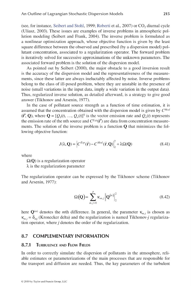
In the case of pollutant source strength as a function of time estimation, it is
assumed that the concentration obtained with the dispersion model is given by C Mod
(r
Æ
, Q), where Q = [Q 1 (t), …, Q n (t)] T is the vector emission rate and Q n (t) represents
the emission rate of the nth source and C Exp (r
Æ
) are data from concentration measurements. The solution of the inverse problem is a function Q that minimizes the following objective function:
2
2
( , )
( )
( , )
( )
Exp
Mod
J
C
C
λ
=
−
+λΩ
Q
r
rQ
Q
(8.41)
where
Ω(Q) is a regularization operator
λ is the regularization parameter
The regularization operator can be expressed by the Tikhonov scheme (Tikhonov
and Arsenin, 1977):
( )
( )
=
Ω
=
κ
∑
2
,
2
, 0
p
m
m j
m j
Q
Q
(8.42)
here Q (m) denotes the mth difference. In general, the parameter κ m.j is chosen as
κ m.j = δ mj (Kronecker delta) and the regularization is named Tikhonov-j regularization operator, where j denotes the order of the regularization.
8.7 COMPLEMENTARY INFORMATION
8.7.1 TURBULENCE AND FLOW FIELDS
In order to correctly simulate the dispersion of pollutants in the atmosphere, reliable estimates or parameterizations of the main processes that are responsible for
the transport and diffusion are needed. Thus, the key parameters of the turbulent
© 2010 by Taylor and Francis Group, LLC
215
(see, for instance, Seibert and Stohl, 1999; Roberti et al., 2007) or CO 2 diurnal cycle
(Uliasz, 2003). These issues are examples of inverse problems in atmospheric pollution modeling (Seibert and Frank, 2004). The inverse problem is formulated as
a nonlinear optimization approach, whose objective function is given by the least
square difference between the observed and prescribed (by a dispersion model) pollutant concentration, associated to a regularization operator. The forward problem
is iteratively solved for successive approximations of the unknown parameters. The
associated forward problem is the solution of the dispersion model.
As pointed out by Seibert (2000), the major obstacle to a good inversion result
is the accuracy of the dispersion model and the representativeness of the measurements, since these latter are always ineluctably affected by noise. Inverse problems
belong to the class of ill-posed problem, where they are unstable in the presence of
noise (small variations in the input data, imply a wide variation in the output data).
Thus, regularized inverse solution, as detailed afterward, is a strategy to give good
answer (Tikhonov and Arsenin, 1977).
In the case of pollutant source strength as a function of time estimation, it is
assumed that the concentration obtained with the dispersion model is given by C Mod
(r
Æ
, Q), where Q = [Q 1 (t), …, Q n (t)] T is the vector emission rate and Q n (t) represents
the emission rate of the nth source and C Exp (r
Æ
) are data from concentration measurements. The solution of the inverse problem is a function Q that minimizes the following objective function:
2
2
( , )
( )
( , )
( )
Exp
Mod
J
C
C
λ
=
−
+λΩ
Q
r
rQ
Q
(8.41)
where
Ω(Q) is a regularization operator
λ is the regularization parameter
The regularization operator can be expressed by the Tikhonov scheme (Tikhonov
and Arsenin, 1977):
( )
( )
=
Ω
=
κ
∑
2
,
2
, 0
p
m
m j
m j
Q
Q
(8.42)
here Q (m) denotes the mth difference. In general, the parameter κ m.j is chosen as
κ m.j = δ mj (Kronecker delta) and the regularization is named Tikhonov-j regularization operator, where j denotes the order of the regularization.
8.7 COMPLEMENTARY INFORMATION
8.7.1 TURBULENCE AND FLOW FIELDS
In order to correctly simulate the dispersion of pollutants in the atmosphere, reliable estimates or parameterizations of the main processes that are responsible for
the transport and diffusion are needed. Thus, the key parameters of the turbulent
© 2010 by Taylor and Francis Group, LLC