

214
Air Pollution and Turbulence: Modeling and Applications
It is important to notice that Equations 8.37a and b collapse on the classical Langevin
equation (for homogeneous turbulence) when m = 0 (see Equation 8.33), that is, when
the wind meandering is absent, namely
d
d
2
u
u
u t
t
u
T
T
Δ
= −
+ σ
ξ
(8.39a)
and
d
d
2
v
v
v t
t
v
T
T
Δ
= −
+ σ
ξ
(8.39b)
Anfossi et al. (2006) applied this new approach (Equation 8.39) in the LSDM for fl at
terrain LAMBDA (Ferrero et al., 1995) to the tracer experiments carried out in low
wind conditions by Idaho National Engineering Laboratory (INEL, Arco, Idaho)
in 1974 (above mentioned) and by the Graz University of Technology and ISAC/
CNR-Turin near Graz in 2003. They found a good agreement between prescribed
and observed ground-level concentrations, and, in particular, found a noticeable
improvement by using Equation 8.39 instead of the standard LAMBDA (not taking
into account the meandering effect).
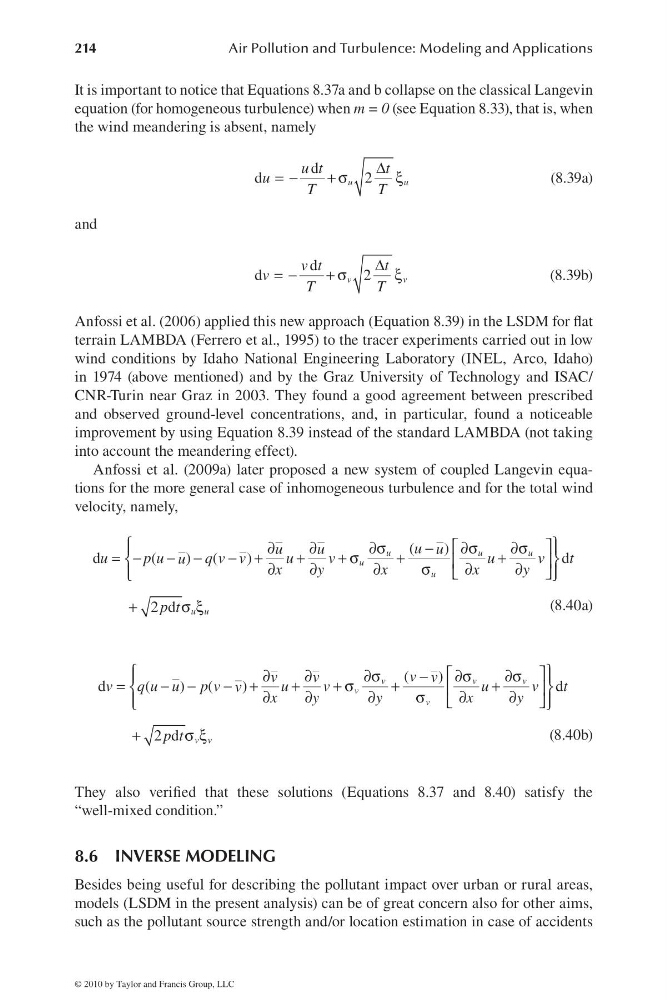
Anfossi et al. (2009a) later proposed a new system of coupled Langevin equations for the more general case of inhomogeneous turbulence and for the total wind
velocity, namely,
⎧
⎫
⎡
⎤
∂
∂
∂σ
−
∂σ
∂σ
⎪
⎪
= −
− −
− +
+
+ σ
+
+
⎨
⎬
⎢
⎥
∂
∂
∂
σ
∂
∂
⎪
⎪
⎣
⎦
⎩
⎭
+
σξ
(
)
d
(
) (
)
d
2 d
u
u
u
u
u
u u
u
u
u
u
u
pu
q v v
u
v
u
v
t
u
x
y
x
x
y
p t
(8.40a)
⎧
⎫
⎡
⎤
∂
∂
∂σ
−
∂σ
∂σ
⎪
⎪
=
− −
− +
+
+σ
+
+
⎨
⎬
⎢
⎥
∂
∂
∂
σ
∂
∂
⎪
⎪
⎣
⎦
⎩
⎭
+
σξ
(
)
d
(
)
(
)
d
2 d
v
v
v
v
v
v v
v
v
v
v
v
q u u p v
u
v
u
v
t
v
x
y
y
x
y
p t
(8.40b)
They also verifi ed that these solutions (Equations 8.37 and 8.40) satisfy the
“ well-mixed condition.”
8.6 INVERSE MODELING
Besides being useful for describing the pollutant impact over urban or rural areas,
models (LSDM in the present analysis) can be of great concern also for other aims,
such as the pollutant source strength and/or location estimation in case of accidents
© 2010 by Taylor and Francis Group, LLC
Air Pollution and Turbulence: Modeling and Applications
It is important to notice that Equations 8.37a and b collapse on the classical Langevin
equation (for homogeneous turbulence) when m = 0 (see Equation 8.33), that is, when
the wind meandering is absent, namely
d
d
2
u
u
u t
t
u
T
T
Δ
= −
+ σ
ξ
(8.39a)
and
d
d
2
v
v
v t
t
v
T
T
Δ
= −
+ σ
ξ
(8.39b)
Anfossi et al. (2006) applied this new approach (Equation 8.39) in the LSDM for fl at
terrain LAMBDA (Ferrero et al., 1995) to the tracer experiments carried out in low
wind conditions by Idaho National Engineering Laboratory (INEL, Arco, Idaho)
in 1974 (above mentioned) and by the Graz University of Technology and ISAC/
CNR-Turin near Graz in 2003. They found a good agreement between prescribed
and observed ground-level concentrations, and, in particular, found a noticeable
improvement by using Equation 8.39 instead of the standard LAMBDA (not taking
into account the meandering effect).
Anfossi et al. (2009a) later proposed a new system of coupled Langevin equations for the more general case of inhomogeneous turbulence and for the total wind
velocity, namely,
⎧
⎫
⎡
⎤
∂
∂
∂σ
−
∂σ
∂σ
⎪
⎪
= −
− −
− +
+
+ σ
+
+
⎨
⎬
⎢
⎥
∂
∂
∂
σ
∂
∂
⎪
⎪
⎣
⎦
⎩
⎭
+
σξ
(
)
d
(
) (
)
d
2 d
u
u
u
u
u
u u
u
u
u
u
u
pu
q v v
u
v
u
v
t
u
x
y
x
x
y
p t
(8.40a)
⎧
⎫
⎡
⎤
∂
∂
∂σ
−
∂σ
∂σ
⎪
⎪
=
− −
− +
+
+σ
+
+
⎨
⎬
⎢
⎥
∂
∂
∂
σ
∂
∂
⎪
⎪
⎣
⎦
⎩
⎭
+
σξ
(
)
d
(
)
(
)
d
2 d
v
v
v
v
v
v v
v
v
v
v
v
q u u p v
u
v
u
v
t
v
x
y
y
x
y
p t
(8.40b)
They also verifi ed that these solutions (Equations 8.37 and 8.40) satisfy the
“ well-mixed condition.”
8.6 INVERSE MODELING
Besides being useful for describing the pollutant impact over urban or rural areas,
models (LSDM in the present analysis) can be of great concern also for other aims,
such as the pollutant source strength and/or location estimation in case of accidents
© 2010 by Taylor and Francis Group, LLC