

An Outline of Lagrangian Stochastic Dispersion Models
213
were satisfactorily tested against the Idaho National Engineering Laboratory (INEL)
tracer dataset (Sagendorf and Dickson, 1974). However, both these models present a
certain amount of empiricism.
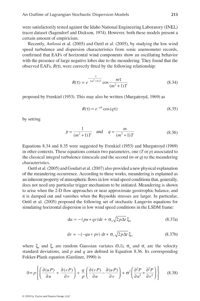
Recently, Anfossi et al. (2005) and Oettl et al. (2005), by studying the low wind
speed turbulence and dispersion characteristics from sonic anemometer records,
confi rmed that EAFs of horizontal wind components show an oscillating behavior
with the presence of large negative lobes due to the meandering. They found that the
observed EAFs, R(τ), were correctly fi tted by the following relationship:
2
(
1 )
2
( )
cos
(
1)
m
T
m
R
e
m
T
τ
−
+
τ
τ =
+
(8.34)
proposed by Frenkiel (1953). This may also be written (Murgatroyd, 1969) as
( )
cos( )
p
R
e
q
− τ
τ =
τ
(8.35)
by setting
2
2
1
and
(
1)
(
1)
m
p
q
m
T
m
T
=
=
+
+
(8.36)
Equations 8.34 and 8.35 were suggested by Frenkiel (1953) and Murgatroyd (1969)
in other contexts. These equations contain two parameters, one (T or p) associated to
the classical integral turbulence timescale and the second (m or q) to the meandering
characteristics.
Oettl et al. (2005) and Goulart et al. (2007) also provided a new physical explanation
of the meandering occurrence. According to these works, meandering is explained as
an inherent property of atmospheric fl ows in low wind speed conditions that, generally,
does not need any particular trigger mechanism to be initiated. Meandering is shown
to arise when the 2-D fl ow approaches or near approximate geostrophic balance, and
it is damped out and vanishes when the Reynolds stresses are larger. In particular,
Oettl et al. (2005) proposed the following set of stochastic Langevin equations for
simulating horizontal dispersion in low wind speed conditions in the LSDM frame:
d
(
)d
2
u
u
u
pu qv t
p t
= −
+
+ σ
Δ ξ
(8.37a)
d
(
)d
2
v
v
v
qu pv t
p t
= − − +
+ σ
Δ ξ
(8.37b)
where ξ u and ξ v are random Gaussian variates (0,1), σ u and σ v are the velocity
standard deviations, and p and q are defi ned in Equation 8.36. Its corresponding
Fokker-Plank equation (Gardiner, 1990) is
2
2
2
2
2
( )
( )
( )
( )
0
u P
v P
q
v P
u P
P
P
p
u
v
p
u
v
u
v
⎧
⎫
⎛
⎞
⎛
⎞
⎛
⎞
∂
∂
∂
∂
∂
∂
⎪
⎪
=
+
+
−
+σ
+
⎨
⎬
⎜
⎟
⎜
⎟
⎜
⎟
∂
∂
∂
∂
∂
∂
⎝
⎠
⎝
⎠
⎝
⎠
⎪
⎪
⎩
⎭
(8.38)
© 2010 by Taylor and Francis Group, LLC
213
were satisfactorily tested against the Idaho National Engineering Laboratory (INEL)
tracer dataset (Sagendorf and Dickson, 1974). However, both these models present a
certain amount of empiricism.
Recently, Anfossi et al. (2005) and Oettl et al. (2005), by studying the low wind
speed turbulence and dispersion characteristics from sonic anemometer records,
confi rmed that EAFs of horizontal wind components show an oscillating behavior
with the presence of large negative lobes due to the meandering. They found that the
observed EAFs, R(τ), were correctly fi tted by the following relationship:
2
(
1 )
2
( )
cos
(
1)
m
T
m
R
e
m
T
τ
−
+
τ
τ =
+
(8.34)
proposed by Frenkiel (1953). This may also be written (Murgatroyd, 1969) as
( )
cos( )
p
R
e
q
− τ
τ =
τ
(8.35)
by setting
2
2
1
and
(
1)
(
1)
m
p
q
m
T
m
T
=
=
+
+
(8.36)
Equations 8.34 and 8.35 were suggested by Frenkiel (1953) and Murgatroyd (1969)
in other contexts. These equations contain two parameters, one (T or p) associated to
the classical integral turbulence timescale and the second (m or q) to the meandering
characteristics.
Oettl et al. (2005) and Goulart et al. (2007) also provided a new physical explanation
of the meandering occurrence. According to these works, meandering is explained as
an inherent property of atmospheric fl ows in low wind speed conditions that, generally,
does not need any particular trigger mechanism to be initiated. Meandering is shown
to arise when the 2-D fl ow approaches or near approximate geostrophic balance, and
it is damped out and vanishes when the Reynolds stresses are larger. In particular,
Oettl et al. (2005) proposed the following set of stochastic Langevin equations for
simulating horizontal dispersion in low wind speed conditions in the LSDM frame:
d
(
)d
2
u
u
u
pu qv t
p t
= −
+
+ σ
Δ ξ
(8.37a)
d
(
)d
2
v
v
v
qu pv t
p t
= − − +
+ σ
Δ ξ
(8.37b)
where ξ u and ξ v are random Gaussian variates (0,1), σ u and σ v are the velocity
standard deviations, and p and q are defi ned in Equation 8.36. Its corresponding
Fokker-Plank equation (Gardiner, 1990) is
2
2
2
2
2
( )
( )
( )
( )
0
u P
v P
q
v P
u P
P
P
p
u
v
p
u
v
u
v
⎧
⎫
⎛
⎞
⎛
⎞
⎛
⎞
∂
∂
∂
∂
∂
∂
⎪
⎪
=
+
+
−
+σ
+
⎨
⎬
⎜
⎟
⎜
⎟
⎜
⎟
∂
∂
∂
∂
∂
∂
⎝
⎠
⎝
⎠
⎝
⎠
⎪
⎪
⎩
⎭
(8.38)
© 2010 by Taylor and Francis Group, LLC